Click here for the MMAB home page Data Analysis using MATLAB and NCTOOLBOX

The following examples use MATLAB^® to extract and visualize the sea surface height from the WAVEWATCH III® model obtained from the NOMADS data server and a downloaded GRiB2 file.

Prerequisites

The examples make use of two free toolboxes,

1. NCTOOLBOX: A MATLAB toolbox for working with common data model datasets
2. M_MAP: A mapping package for MATLAB.

• Example 1: Plot data from the NOMADS Data Server
• Example 2: Plot data from a WAVEWATCH III^® GRiB file

Example 1: Plot data from the NOMADS Data Server

% First set up the URL to access the data server.
% See the WAVEWATCH III® multi-grid directory on NOMADS 
% for the list of available model run dates.

mydate='20231203';
url=['//nomads.ncep.noaa.gov:9090/dods/wave/mww3/',mydate, ...
     '/multi_1.glo_30mext',mydate,'_00z'];

% Instantiate the data set
nco=ncgeodataset(url);

% Extract the longitude and latitude vectors and the surface 
% significant height of wind waves from NOMADS.

lon=nco{'lon'}(:);
lat=nco{'lat'}(:);
waveheight=nco{'htsgwsfc'}(1,:,:);

% The indexing into the data set is standard MATLAB array indexing.
% We need to convert the data from single to double precision and remove
% any singleton dimensions, as the NCTOOLBOX routines return the numbers 
% as they are stored in the netCDF file, in this case single precision.

waveheight=double(squeeze(waveheight));
lat=double(lat);
lon=double(lon);

% Plot the field using M_MAP.  Start with setting the map
% projection using the limits of the lat/lon data itself:

m_proj('miller','lat',[min(lat(:)) max(lat(:))],...
'lon',[min(lon(:)) max(lon(:))])

% Next, plot the field using the M_MAP version of pcolor.

m_pcolor(lon,lat,waveheight);
shading flat;

% Add a coastline and axis values.

m_coast('patch',[.7 .7 .7])
m_grid('box','fancy')

% Add a colorbar and title.

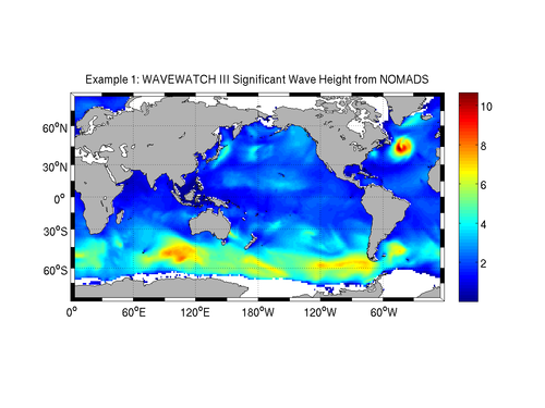
colorbar
title('Example 1: WAVEWATCH III Significant Wave Height from NOMADS');

This example requires that you download a GRiB file from either our NOMADS data server or the Production FTP Server (see our Model Data Access page for more information. The GRiB files for the latest runs can be found here: nomads.ncep.noaa.gov/pub/data/nccf/com/wave/prod/. Look in the directories prefixed by "multi_1.".

For this exercise, I used a production nowcast file for the 10 arc-minute grid for the US East Coast: multi_1.at_10m.t00z.f000.grib2 retrieved from NOMADS. This example assumes that the GRiB file is in the current working directory.

Note that the file variables have different names when you access it locally instead of through the OpenDAP interface. Specifically, "sshgsfc" becomes "Sea_Surface_Height_Relative_to_Geoid", "lat" is "Latitude_of_Presure_Point_surface" and "lon" is "Longitude_of_Presure_Point_surface". Once you've defined the ncgeodataset (in this case called nco), you can examine the variable names by printing out the values of nco.variables. Note that since we are working with the model's native grid (Arakawa C-Grid) the lat/lon positions for some values (ssh, temperature, mixed layer depth, others) is different from the lat/lon points for the horizontal velocity components.

grib=' multi_1.at_10m.t00z.f000.grib2';

nco=ncgeodataset(grib);
nco.variables
ans = 
    'Wind_direction_from_which_blowing_degree_true_surface'
    'Wind_speed_surface'
    'u-component_of_wind_surface'
    'v-component_of_wind_surface'
    'Significant_height_of_combined_wind_waves_and_swell_surface'
    'Direction_of_wind_waves_degree_true_surface'
    'Significant_height_of_wind_waves_surface'
    'Mean_period_of_wind_waves_surface'
    'Direction_of_swell_waves_degree_true_ordered_sequence_of_data'
    'Significant_height_of_swell_waves_ordered_sequence_of_data'
    'Mean_period_of_swell_waves_ordered_sequence_of_data'
    'Primary_wave_direction_degree_true_surface'
    'Primary_wave_mean_period_surface'
    'lat'
    'lon'
    'ordered_sequence_of_data'
    'time'

% Extract the Significant Height of Swell Waves field.

param='Significant_height_of_swell_waves_ordered_sequence_of_data';
waveheight=nco{param}(1,1,:,:);
lat=nco{'lat'}(:);
lon=nco{'lon'}(:);

% From this point on the code is identical to the previous example:

waveheight=double(squeeze(waveheight));
lat=double(lat);
lon=double(lon);
m_proj('miller','lat',[min(lat(:)) max(lat(:))],...
  'lon',[min(lon(:)) max(lon(:))])
m_pcolor(lon,lat,waveheight);
shading flat;
m_coast('patch',[.7 .7 .7]);
m_grid('box','fancy')
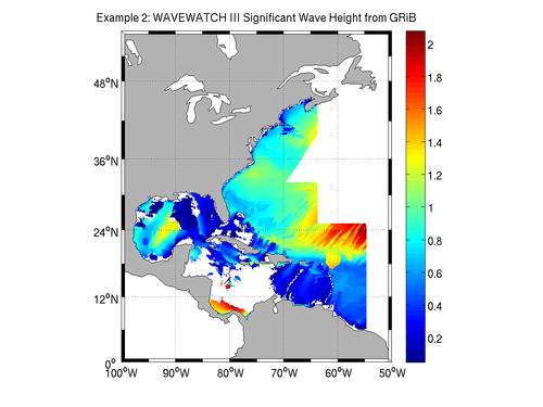
colorbar
title('Example 2: WAVEWATCH III Significant Wave Height from GRiB');