Click here to go to the MMAB homepage Examples of RTOFS Atlantic Model Data Processing with Python

The following examples use Sage Python to extract and visualize the sea surface height and ocean temperature in the RTOFS Atlantic model using data from the NOMADS data server and a downloaded RTOFS GRiB file.

Prerequisites

The examples make use of the following free software:

1. SAGE Open Source Mathematics Software
2. pygrib2: A module for reading and writing GRIB Edition 2 files
3. netcdf4-python: A Python/numpy interface to netCDF
4. Basemap: A module to plot data on map projections with matplotlib

• Example 1: Plot data from the NOMADS Data Server
• Example 2: Plot data from an RTOFS GRiB file

Example 1: Plot data from the NOMADS Data Server

Begin by importing the necessary modules and set up the figure

from mpl_toolkits.basemap import Basemap
import numpy as np
import matplotlib.pyplot as plt
from pylab import *
import netCDF4

plt.figure()

First set up the URL to access the data server. See the RTOFS directory on NOMADS for the list of available model run dates.

mydate='20250329';
url='http://nomads.ncep.noaa.gov:9090/dods/ofs/ofs'+ \
  mydate+'/hourly/rtofs_forecast_atl'

Note that the NOMADS data server interpolates and delivers the data on a regular lat/lon field, not the native model grid. To analyze the model output on the native grid you will have to work from a downloaded GRiB file (see Example 2).

Extract the sea surface height field from NOMADS.

file = netCDF4.Dataset(url)
lat  = file.variables['lat'][:]
lon  = file.variables['lon'][:]
data      = file.variables['sshgsfc'][1,:,:]
file.close()

Since Python is object oriented, you can explore the contents of the NOMADS data set by examining the file object, such as file.variables.

The indexing into the data set used by netCDF4 is standard python indexing. In this case we want the first forecast step, but note that the first time step in the RTOFS OpenDAP link is all NaN values. So we start with the second timestep.

Plot the field using Basemap. Start with setting the map projection using the limits of the lat/lon data itself:

m=Basemap(projection='mill',lat_ts=10,llcrnrlon=lon.min(), \
  urcrnrlon=lon.max(),llcrnrlat=lat.min(),urcrnrlat=lat.max(), \
  resolution='c')

Convert the lat/lon values to x/y projections.

Lon, Lat = meshgrid(lon,lat)
x, y = m(Lon,Lat)

Next, plot the field using the fast pcolormesh routine and set the colormap to jet.

cs = m.pcolormesh(x,y,data,shading='flat',cmap=plt.cm.jet)

Add a coastline and axis values.

m.drawcoastlines()
m.fillcontinents()
m.drawmapboundary()
m.drawparallels(np.arange(-90.,120.,30.),labels=[1,0,0,0])
m.drawmeridians(np.arange(-180.,180.,60.),labels=[0,0,0,1])

Add a colorbar and title, and then show the plot.

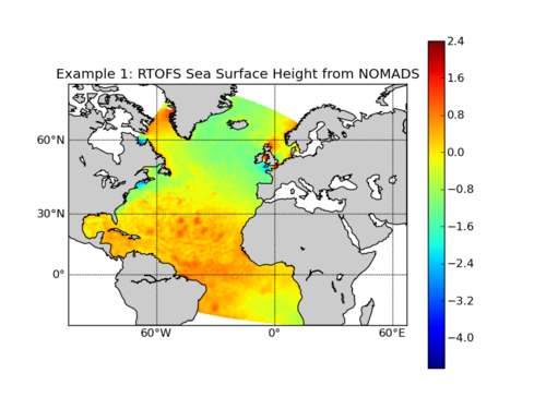
colorbar(cs,orientation='vertical')
plt.title('Example 1: RTOFS Sea Surface Height from NOMADS')
plt.show()

You should see this image in your figure window:

---

Example 2: Plot data from an RTOFS GRiB file

This example requires that you download a GRiB file from either our NOMADS data server or the Production FTP Server (see our Data Access page for more information. For this exercise, I used the nowcast file for 20111004: ofs_atl.t00z.N000.grb.grib2 retrieved from NOMADS. This example assumes that the GRiB file is in the current working directory.

Begin by importing the necessary modules and set up the figure

from grib2 import Grib2Decode
from mpl_toolkits.basemap import Basemap
import matplotlib.pyplot as plt
from pylab import *

plt.figure()

grib='ofs_atl.t00z.N000.grb.grib2';

Note that the file variables have different names when you access it locally instead of through the OpenDAP interface. Due to external table definition issues with the GRiB-2 files created by RTOFS-Atlantic, the parameter names are a little troublesome. In this example we match against the full parameter names instead of the abbreviated names. For example, "WTMPC" as reported by the wgrib2 utility is identified as "3-D Temperature" in the full parameter name field. Additionally, we will need to extract the lat/lon fields from the extra fields at the end of the GRiB file instead of using the GRiB header based grid information. Note that since we are working with the model's native grid (Arakawa C-Grid) the lat/lon positions for some values (ssh, temperature, mixed layer depth, others) is different from the lat/lon points for the horizontal velocity components. And note that there is a slight misspelling in the pressure point latitude and longitude parameter names.

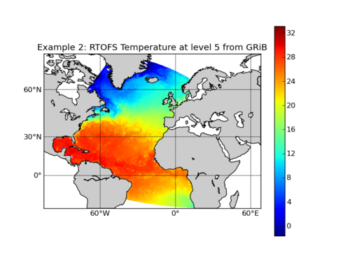
In this example we will extract the temperature field from the 5^th level in the model. Remember that indexing in Python starts at zero.

want_level = 4
zgribs = [g for g in grbs if g.parameter == '3-D Temperature']
nlevs = len(zgribs)
for nlev,zg in enumerate(zgribs):
    if nlev == want_level: temp = zg.data()
    
for g in grbs:
  if g.parameter == 'Longitude of Presure Point':
    lon = g.data()
  if g.parameter == 'Latitude of Presure Point':
    lat = g.data()

From this point on the code is almost identical to the previous example. The missing step is that since lat/lon values are arrays in the native grid instead of vectors returned by NOMADS, the meshgrid step is unnecessary.

Plot the field using Basemap. Start with setting the map projection using the limits of the lat/lon data itself:

m=Basemap(projection='mill',lat_ts=10,llcrnrlon=lon.min(), \
  urcrnrlon=lon.max(),llcrnrlat=lat.min(),urcrnrlat=lat.max(), \
  resolution='c')

Convert the lat/lon values to x/y projections.

x, y = m(lon,lat)

Next, plot the field using the fast pcolormesh routine and set the colormap to jet.

cs = m.pcolormesh(x,y,data,shading='flat',cmap=plt.cm.jet)

Add a coastline and axis values.

m.drawcoastlines()
m.fillcontinents()
m.drawmapboundary()
m.drawparallels(np.arange(-90.,120.,30.),labels=[1,0,0,0])
m.drawmeridians(np.arange(-180.,180.,60.),labels=[0,0,0,1])

Add a colorbar and title, and then show the plot.

colorbar(cs,orientation='vertical')
plt.title('Example 2: RTOFS Temperature at level 5 from GRiB')
plt.show()

You should see this image in your figure window: