Example 1: Plot data from the NOMADS Data Server
First set up the URL to access the data server.
See the
RTOFS directory on NOMADS for the list of available model run dates.
-
mydate='20251214';
url=['http://nomads.ncep.noaa.gov:9090/dods/ofs/ofs',...
   mydate,'/hourly/rtofs_forecast_atl'];
The contents of the OpenDAP dataset can be explored by clicking on the
"Info" button in the RTOFS directory for the day or by using this command in
MATLAB:
-
nj_info(url)
Note that the NOMADS data server interpolates and delivers the data on a
regular lat/lon field, not the native model grid. To analyze the model
output on the native grid you will have to work from a downloaded GRiB file
(see Example 2).
Extract the sea surface height field from NOMADS.
-
nco=ncgeodataset(url);
ssh=nco{'sshgsfc'}(2,1,:,:);
lon=nco{'lon'}(:);
lat=nco{'lat'}(:);
The indexing into the data set is standard MATLAB array indexing. In
this case we want the first forecast step, but note that the first
time step in the RTOFS OpenDAP link is all NaN values. So we start
with the second timestep.
We need to convert the data from single to double precision and remove
any singleton dimensions, as the
NCTOOLBOX routines return the numbers as they are stored in the netCDF
file, in this case single precision.
-
ssh=double(squeeze(ssh));
lat=double(lat);
lon=double(lon);
Plot the field using M_MAP. Start with setting the map
projection using the limits of the lat/lon data itself:
-
m_proj('miller','lat',[min(lat(:)) max(lat(:))],...
'lon',[min(lon(:)) max(lon(:))])
Next, plot the field using the M_MAP version of pcolor.
-
m_pcolor(lon,lat,ssh);
shading flat;
Add a coastline and axis values.
-
m_coast('patch',[.7 .7 .7])
m_grid('box','fancy')
Add a colorbar and title.
-
colorbar
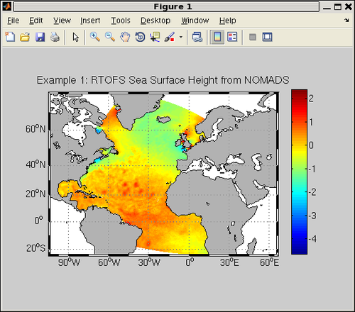
title('Example 1: RTOFS Sea Surface Height from NOMADS');
You should see this image in your figure window:
Example 2: Plot data from an RTOFS GRiB file
This example requires that you download a GRiB file from either our NOMADS
data server or the Production FTP Server (see our
Data Access page
for more information. For this exercise, I used the
nowcast file for 20111004: ofs_atl.t00z.N000.grb.grib2 retrieved from
NOMADS. This example assumes that the GRiB file is in the current working directory.
-
grib='ofs_atl.t00z.N000.grb.grib2';
Note that the file variables have different names when you access it locally
instead of through the OpenDAP interface. Specifically, "sshgsfc" becomes
"Sea_Surface_Height_Relative_to_Geoid", "lat" is
"Latitude_of_Presure_Point_surface" and "lon" is
"Longitude_of_Presure_Point_surface". Once you've defined the
ncgeodataset (in this case called nco), you can examine the variable
names by printing out the values of nco.variables.
Note that since we are working with the model's native grid (Arakawa C-Grid)
the lat/lon positions for some values (ssh, temperature, mixed layer depth,
others) is different from the lat/lon points for the horizontal velocity
components.
-
nco=ncgeodataset(grib);
nco.variables
And now we extract the SSH field using the parameter names from nj_info:
-
ssh=nco{'Sea_Surface_Height_Relative_to_Geoid_surface'}(1,1,:,:);
lat=nco{'Latitude_of_Presure_Point_surface'}(:);
lon=nco{'Longitude_of_Presure_Point_surface'}(:);
Note that because each GRiB file has only a single time step I access the
first time point, not the second as was the case in Example 1.
From this point on the code is identical to the previous example:
-
ssh=double(squeeze(ssh));
lat=double(lat);
lon=double(lon);
m_proj('miller','lat',[min(lat(:)) max(lat(:))],...
'lon',[min(lon(:)) max(lon(:))])
m_pcolor(lon,lat,ssh);
shading flat;
m_coast('patch',[.7 .7 .7]);
m_grid('box','fancy')
colorbar
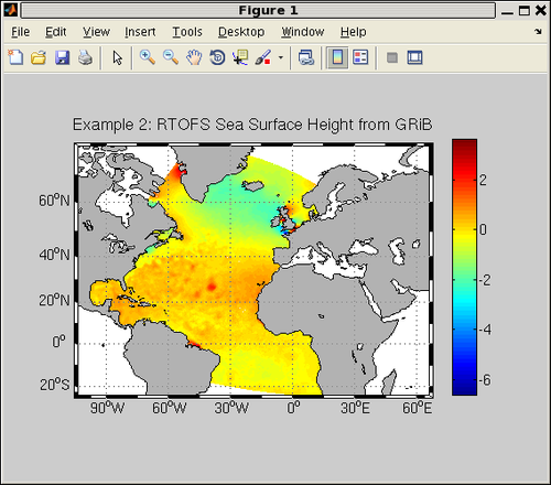
title('Example 2: RTOFS Sea Surface Height from GRiB');
You should see this image in your figure window:
MATLAB® is a registered trademark of The Mathworks. Inc.