Global RTOFS Data Analysis with MATLAB and NCTOOLBOX

Home Z-Levels Fronts Sea Ice Metrics DA QC (internal use) Data Access About

The following examples use MATLAB® to extract and visualize the sea surface temperature of the Global RTOFS model using the NOMADS data server and a downloaded NetCDF file.

Prerequisites

The examples make use of two free toolboxes,

1. NCTOOLBOX for MATLAB
2. M_MAP: A mapping package for MATLAB.

These toolboxes can be installed in your home directory, they do not need to be installed into the system-wide folders. Note that the NCTOOLBOX can read NetCDF, OPeNDAP, HDF5, GRIB, GRIB2, HDF4 and many (15+) other file formats and services using the same API.

Example: Plot data from the NOMADS Data Server or a local NetCDF file

To extract data directly from the NOMADS, first set up the URL to access the data server. See the Global RTOFS directory on NOMADS for the list of available model run dates.

If you have downloaded a NetCDF file of Global RTOFS data from NOMADS or the NCO Production FTP server (FTPPRD), then you simply set the url variable to point to the local NetCDF file. The rest of the example procedure is exactly the same regardless of the source of the data.

mydate='20250702';
url=['//nomads.ncep.noaa.gov:9090/dods/',...
  'rtofs/rtofs_global',mydate,...
  '/rtofs_glo_3dz_nowcast_daily_temp'];

url='rtofs_glo_3dz_n048_daily_3ztio.nc';

url='rtofs_glo_3dz_n048_daily_3ztio.nc';

If you're accessing the NOMADS OpenDAP url, then the contents of the OpenDAP dataset can be explored by clicking on the "Info" button in the Global RTOFS directory for the day. Or you can examine the contents of the OpenDAP url or a local NetCDF file by using this command in MATLAB:

nc = ncgeodataset(url);
info = nc.metadata

This returns a MATLAB structure containing fields representing global and variable attributes of the dataset. To access a list of variable names and the array size of a particular variable do the following:

var_list = nc.variables
siz = nc.size(‘temperature’))

Note that the NOMADS data server interpolates and delivers the data on a regular lat/lon field, not the native model grid. To obtain model data on the native grid you can either download the NetCDF file or use one of the experimental NOPDEF OpenDAP urls available from the Developmental NOMADS server (look for "NOPDEF" in the directory name for the model run day). The NOPDEF url skips the interpolation step and delivers the Global RTOFS data on its native tripolar grid. Note that in that case the latitude and longitude values are returned as arrays instead of vectors.

Extract the sea surface temperature field from NOMADS. There are several different methods that can be used in NCTOOLBOX to retrieve data:

nc = ncgeodataset(url);

% method 1:
siz = nc.size(‘temperature’);
sst = nc.data(‘temperature’, [2 1 1 1],[2 1 siz(3) siz(4)]);
lon = nc.data(‘lon’);
lat = nc.data(‘lat’);

% method 2:  
      
var = nc.geovariable(‘temperature’);
sst = var.data(2, 1, :, :);
                  
% method 3:
                        
sst = nc{‘temperature’}(2, 1, :, :);
lon = nc{‘lon’}(:);
lat = nc{‘lat’}(:);

The first method uses a "hyperslab" scheme where one-based indexing is used to specify a starting corner (start_time,lon,lat) and an ending corner (stop_time,lon,lat). The second method first creates a variable object, which allows allows Matlab-style indexing as well as some more powerful capabilities (see NCTOOLBOX documentation for more information). The third method uses curly braces to streamline access, and also uses Matlab-style indexing.

Note that we want the first forecast step, but the first time step in the Global RTOFS OpenDAP link is all NaN values. So we start with the second timestep.

Important Note: There is a gotcha in the longitude field. The model does not use the rightmost column in the longitude grid and consequently it fills it with large non-zero values (typically > 500). We mask those points out with NaNs.

sst=squeeze(double(sst));
lat=double(lat);
lon=double(lon);
lon(end,:)=nan;

m_proj('miller',...
  'lat',[min(lat(:)) max(lat(:))],...
  'lon',[min(lon(:)) max(lon(:))])

m_pcolor(lon,lat,sst);
shading flat;

m_coast('patch',[.7 .7 .7])
m_grid('box','fancy')

colorbar
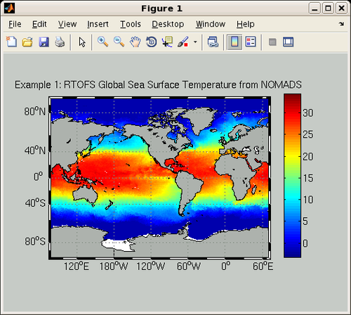
title('Example 1: Global RTOFS SST from NOMADS');

Additional Notes on using MATLAB

The sheer size of the data structures and arrays can cause MATLAB to throw a Java Out of Memory error, particularly when reading an external data file with one of the toolboxes that uses the NetCDF for Java libraries. In this case it is necessary to increase the Java Virtual Machine heap memory allocation. For most purposes, we've found that increasing the Java heap space allocation to 256MB with a maximum value of 6GB is adequate for our needs. This presumes that sufficient memory is available for such a high setting, and can depend on the physical memory limits in your system.