Examples of NWW3 Model Data Processing with Python (Text)

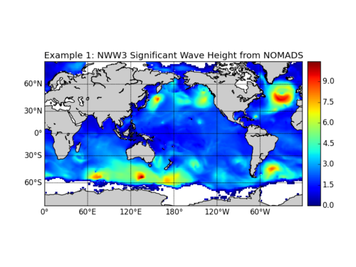
The following examples use Python to extract and visualize the sea surface height and ocean temperature in the NWW3 model using data from the NOMADS data server and a downloaded NWW3 GRiB2 file.

Prerequisites

The examples make use of the following free software:

1. Python
2. Numpy (Numerical Python
3. netcdf4-python: A Python/numpy interface for NetCDF and OpenDAP
4. Basemap: A module to plot data on map projections with matplotlib
5. pygrib (python module for reading GRiB files)

• Example 1: Plot data from the NOMADS Data Server
• Example 2: Plot data from an NWW3 GRiB2 file

# basic NOMADS OpenDAP extraction and plotting script
from mpl_toolkits.basemap import Basemap
import numpy as np
import matplotlib.pyplot as plt
import netCDF4

# set up the figure
plt.figure()

# set up the URL to access the data server.
# See the NWW3 directory on NOMADS 
# for the list of available model run dates.

mydate='20240426'
url='//nomads.ncep.noaa.gov:9090/dods/wave/nww3/nww3'+ \
    mydate+'/nww3'+mydate+'_00z'

# Extract the significant wave height of combined wind waves and swell

file = netCDF4.Dataset(url)
lat  = file.variables['lat'][:]
lon  = file.variables['lon'][:]
data = file.variables['htsgwsfc'][1,:,:]
file.close()

# Since Python is object oriented, you can explore the contents of the NOMADS
# data set by examining the file object, such as file.variables.

# The indexing into the data set used by netCDF4 is standard python indexing.
# In this case we want the first forecast step, but note that the first time 
# step in the RTOFS OpenDAP link is all NaN values.  So we start with the 
# second timestep

# Plot the field using Basemap.  Start with setting the map
# projection using the limits of the lat/lon data itself:

m=Basemap(projection='mill',lat_ts=10,llcrnrlon=lon.min(), \
  urcrnrlon=lon.max(),llcrnrlat=lat.min(),urcrnrlat=lat.max(), \
  resolution='c')

# convert the lat/lon values to x/y projections.

x, y = m(*np.meshgrid(lon,lat))

# plot the field using the fast pcolormesh routine 
# set the colormap to jet.

m.pcolormesh(x,y,data,shading='flat',cmap=plt.cm.jet)
m.colorbar(location='right')

# Add a coastline and axis values.

m.drawcoastlines()
m.fillcontinents()
m.drawmapboundary()
m.drawparallels(np.arange(-90.,120.,30.),labels=[1,0,0,0])
m.drawmeridians(np.arange(-180.,180.,60.),labels=[0,0,0,1])

# Add a colorbar and title, and then show the plot.

plt.title('Example 1: NWW3 Significant Wave Height from NOMADS')
plt.show()

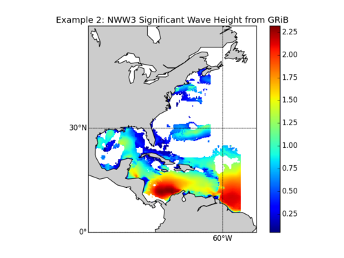
This example requires that you download a GRiB2 file from either our NOMADS data server or the Production FTP Server (see our Data Access page for more information. For this exercise, I used the file multi_1.at_10m.t00z.f000.grib2 retrieved from NOMADS. This example assumes that the GRiB2 file is in the current working directory.

Begin by importing the necessary modules and set up the figure

import numpy as np
import pygrib
import matplotlib.pyplot as plt
from mpl_toolkits.basemap import Basemap

plt.figure()

grib='multi_1.at_10m.t00z.f000.grib2';
grbs=pygrib.open(grib)

In this example we will extract the same significant wave height field we used in the first example. Remember that indexing in Python starts at zero.

grb = grbs.select(name='Significant height of wind waves')[0]
data=grb.values
lat,lon = grb.latlons()

From this point on the code is almost identical to the previous example.

Plot the field using Basemap. Start with setting the map projection using the limits of the lat/lon data itself:

m=Basemap(projection='mill',lat_ts=10,llcrnrlon=lon.min(), \
  urcrnrlon=lon.max(),llcrnrlat=lat.min(),urcrnrlat=lat.max(), \
  resolution='c')

Convert the lat/lon values to x/y projections.

x, y = m(lon,lat)

Next, plot the field using the fast pcolormesh routine and set the colormap to jet.

cs = m.pcolormesh(x,y,data,shading='flat',cmap=plt.cm.jet)

Add a coastline and axis values.

m.drawcoastlines()
m.fillcontinents()
m.drawmapboundary()
m.drawparallels(np.arange(-90.,120.,30.),labels=[1,0,0,0])
m.drawmeridians(np.arange(-180.,180.,60.),labels=[0,0,0,1])

Add a colorbar and title, and then show the plot.

plt.colorbar(cs,orientation='vertical')
plt.title('Example 2: NWW3 Significant Wave Height from GRiB')
plt.show()