Todd Spindler
IMSG at NCEP/EMC
Verification Post Processing Product Generation Branch
Learn scientific data visualization in three easy* lessons!
* and many more perhaps not-quite-so-easy lessons...
Just an FYI before we begin
This entire presentation was created using Python 3 and Jupyter Notebooks
All three example notebooks and the data sets are available from our web site:
Feel free to download them and play with the notebooks
Three commonly used binary dataset formats in use at EMC are (in no particular order):
NetCDF (Network Common Data Format)
GRIB (GRIdded Binary or General Regularly-distributed Information in Binary form)
BUFR (Binary Universal Form for the Representation of meteorological data)
Example 1: Reading a NetCDF data set
NetCDF can be read with any of the following libraries:
netCDF4-python
xarray
PyNIO
In this example we'll use xarray to read a Global RTOFS NetCDF dataset, plot a parameter (SST), and select a subregion.
The xarray library can be installed via pip, conda (or whatever package manager comes with your Python installation), or distutils (python setup.py).
- Begin by importing the required libraries.
import matplotlib.pyplot as plt    # standard graphics library
import xarray
import cartopy.crs as ccrs         # cartographic coord reference system
import cartopy.feature as cfeature # features: land, borders, coastlines
- Open the file as an xarray Dataset and display the metadata.
dataset = xarray.open_dataset('rtofs_glo_2ds_n000_daily_prog.nc',
                              decode_times = True)
decode_times = Truewill automatically decode the datetime values from NetCDF convention to Python datetime objectsNote that this reads a local data set, but you can replace the filename with the URL of the corresponding NOMADS OpenDAP data set and continue without further changes.
dataset
- There's an extra Date field. Since it's not needed, here's how to get rid of it.
dataset = dataset.drop('Date')
- You can also use the python delete command:
del dataset['Date']
There's a quirk in the Global RTOFS datasets -- the bottom row of the longitude field is unused by the model and is filled with junk data.
I'll use array subsetting to get rid of it, and save just the SST parameter to a separate DataArray.
sst = dataset.sst[0,0:-1,:] # this can be shortened to [0,:-1,]
- Note that subsetting an xarray parameter will also subset the associated coordinates at the same time.
sst
- For a quick look at the raw data array, use matplotlib's
imshowfunction to display the SST parameter as an image.
plt.figure(dpi = 90)         # open a new figure window and set the resolution
plt.imshow(sst, cmap = 'gist_ncar');

- This is how the model data is stored in the array. The Latitude array is similarly upside down.
- Also note that the longitude values are a bit odd.
print(sst.Longitude.min().data, sst.Longitude.max().data)
- In fact, the whole model grid is pretty weird. It's called a tripolar grid.
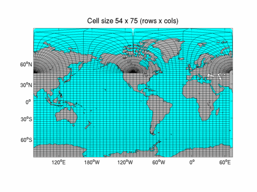
- Now set up the figure and plot the SST field in a Mercator projection, using Cartopy to handle the projection details and letting xarray decide how to plot the data. The default for 2-D plotting is
pcolormesh().
- Xarray is very smart and will try to use a diverging (bicolor) colormap if the data values straddle zero.
- You override this by specifying the colormap with
cmap=and thevmin=, vmax=values for your data.
plt.figure(dpi = 100)
ax = plt.axes(projection = ccrs.Mercator())
ax.add_feature(cfeature.LAND)           # fill in the land areas
ax.coastlines()                         # use the default coastline
gl = ax.gridlines(draw_labels = True)   # default is to label all axes.
gl.xlabels_top = False                  # turn off two of them.
gl.ylabels_right = False

sst.plot(x = 'Longitude', y = 'Latitude', cmap = 'gist_ncar',
         vmin = sst.min(), vmax=sst.max(),
         transform = ccrs.PlateCarree());

- Now let's concentrate on the waters around Hawaii (lat: 17 to 24, lon: -163 to -153)
- RTOFS longitudes are defined as 74-430, so we need to convert the -163 and -153 values by computing modulo 360. Python uses the "%" operator for modulus math.
- Use the
object.where()method with the lat/lon limits.
hawaii = sst.where((sst.Longitude >= -163%360) &
                   (sst.Longitude <= -153%360) &
                   (sst.Latitude >= 17) &
                   (sst.Latitude <= 24), drop = True)
- Note the
drop = Trueoption, which instructs the.where()method to subset the data. Otherwise it will retain the full array size and simply mask out the unwanted data.
- As before, let's plot the SST in a Mercator projection, but use a high-resolution coastline.
- Since the water around Hawaii is warm I don't have to specify the colormap limits.
plt.figure(dpi = 100)
ax = plt.axes(projection = ccrs.Mercator())
ax.add_feature(cfeature.LAND)
ax.add_feature(cfeature.GSHHSFeature()) # use a high-resolution GSHHS coastline
gl = ax.gridlines(draw_labels=True)
gl.xlabels_top = False
gl.ylabels_right = False

hawaii.plot.contourf(x = 'Longitude',y = 'Latitude',levels = 20,
                     cmap = 'gist_ncar',add_colorbar = True,
                     transform = ccrs.PlateCarree());
