Time Series Data Analysis with Python

Deanna Spindler

IMSG at NCEP/EMC
Verification, Post-Processing and Product Generation Branch

What is pandas?

The name comes from panel data, a statistics term for multidimensional datasets.

A high-perfomance open source library for tabular data manipulation and analysis developed by Wes McKinney in 2008.

What does it do?

  • Process a variety of data sets in different formats: time series,
    heterogeneous tables, and matrix data.
  • Provides a suite of data structures:
    • Series (1D => think columns),
    • DataFrame (2D => think tables or spreadsheets)
    • Panel (3D => a matrix of tables, I prefer to just use xarray)
  • Missing data can be ignored, converted to 0, etc
  • Facilitates many operations: subsetting, slicing, filtering, merging,
    grouping, re-ordering and re-shaping
  • Integrates well with other Python libraries, such as statsmodels and SciPy
  • Easily load/import data from CSV and DB/SQL

Example

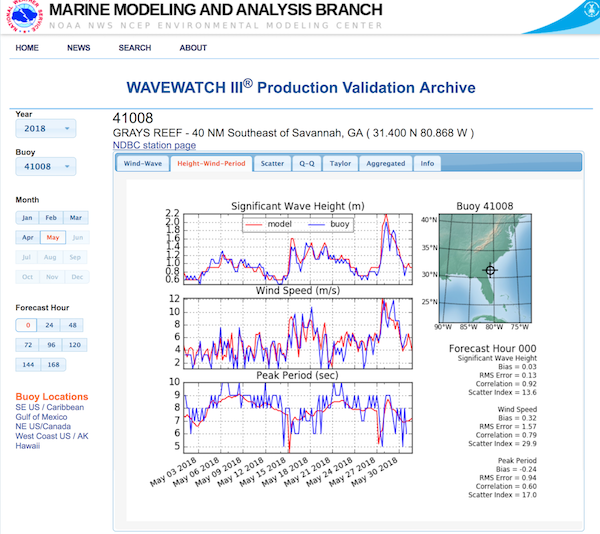
Using pandas DataFrames to validate WAVEWATCH III model output with NDBC buoy data.

  • Creating DataFrames from ASCII files and remote data servers (OPeNDAP)

  • DataFrame manipulations (selecting, merging, grouping)

  • Basic descriptive statistics (RMS, Bias, Cross-Correlation, Scatter Index)

First things first

In [2]:
import matplotlib.pyplot as plt
import numpy
import pandas
import tarfile
import xarray 
import netCDF4
from datetime import datetime,timedelta
from dateutil.relativedelta import relativedelta

Start by choosing a buoy and period of interest

In [3]:
buoyID='41008'
year=2018
month=6

Get the quality controlled NDBC data

In [4]:
url='https://dods.ndbc.noaa.gov/thredds/dodsC/data/stdmet/'+buoyID+'/'+ \
    buoyID+'h'+str(year)+'.nc'
ncdata=xarray.open_dataset(url,decode_times=True)

Select the specific month of the year

In [5]:
startat=datetime(year,month,1)
stopat=startat+relativedelta(months=1)-relativedelta(days=1)

Subset the data to this time period, and make it a DataFrame

In [6]:
data=ncdata.sel(time=slice(startat,stopat)).to_dataframe()

Take a look at what is there

In [7]:
data.keys()
Out[7]:
Index(['wind_dir', 'wind_spd', 'gust', 'wave_height', 'dominant_wpd',
       'average_wpd', 'mean_wave_dir', 'air_pressure', 'air_temperature',
       'sea_surface_temperature', 'dewpt_temperature', 'visibility',
       'water_level'],
      dtype='object')

Another way is to look at the first few rows of the DataFrame

In [8]:
data.head()
Out[8]:
wind_dir wind_spd gust wave_height dominant_wpd average_wpd mean_wave_dir air_pressure air_temperature sea_surface_temperature dewpt_temperature visibility water_level
latitude longitude time
31.4 -80.867996 2018-06-01 00:50:00 172.0 8.2 9.4 0.80 00:00:07.690000 00:00:03.950000 100.0 1014.500000 25.700001 26.100000 NaN NaN NaN
2018-06-01 01:50:00 178.0 7.5 8.5 0.89 00:00:07.140000 00:00:03.940000 109.0 1015.200012 25.700001 25.799999 NaN NaN NaN
2018-06-01 02:50:00 186.0 7.0 8.2 0.80 00:00:07.690000 00:00:03.900000 113.0 1015.200012 25.700001 25.700001 NaN NaN NaN
2018-06-01 03:50:00 200.0 6.9 8.8 0.86 00:00:07.690000 00:00:04.160000 103.0 1015.299988 25.799999 25.600000 NaN NaN NaN
2018-06-01 04:50:00 205.0 6.3 7.3 0.79 00:00:03.700000 00:00:04.080000 171.0 1014.799988 25.600000 25.600000 NaN NaN NaN

I like to index on a datetime stamp, so let's reset the index

In [9]:
data=data.reset_index()
data.index=data['time'].dt.round('1H')
data.index.name='datetime'
In [10]:
data.head()
Out[10]:
latitude longitude time wind_dir wind_spd gust wave_height dominant_wpd average_wpd mean_wave_dir air_pressure air_temperature sea_surface_temperature dewpt_temperature visibility water_level
datetime
2018-06-01 01:00:00 31.4 -80.867996 2018-06-01 00:50:00 172.0 8.2 9.4 0.80 00:00:07.690000 00:00:03.950000 100.0 1014.500000 25.700001 26.100000 NaN NaN NaN
2018-06-01 02:00:00 31.4 -80.867996 2018-06-01 01:50:00 178.0 7.5 8.5 0.89 00:00:07.140000 00:00:03.940000 109.0 1015.200012 25.700001 25.799999 NaN NaN NaN
2018-06-01 03:00:00 31.4 -80.867996 2018-06-01 02:50:00 186.0 7.0 8.2 0.80 00:00:07.690000 00:00:03.900000 113.0 1015.200012 25.700001 25.700001 NaN NaN NaN
2018-06-01 04:00:00 31.4 -80.867996 2018-06-01 03:50:00 200.0 6.9 8.8 0.86 00:00:07.690000 00:00:04.160000 103.0 1015.299988 25.799999 25.600000 NaN NaN NaN
2018-06-01 05:00:00 31.4 -80.867996 2018-06-01 04:50:00 205.0 6.3 7.3 0.79 00:00:03.700000 00:00:04.080000 171.0 1014.799988 25.600000 25.600000 NaN NaN NaN

The parameter names are long, and there are columns that are not used.

Let's fix that

In [11]:
params={'wind_dir':'udir',
        'wind_spd':'u10',
        'wave_height':'Hs',
        'dominant_wpd':'Tp',
        'longitude':'lon',
        'latitude':'lat'}
dropkeys=[key for key in data if key not in params]
data.drop(dropkeys,axis=1,inplace=True)
data.rename(columns=params,inplace=True)
In [12]:
data.head()
Out[12]:
lat lon udir u10 Hs Tp
datetime
2018-06-01 01:00:00 31.4 -80.867996 172.0 8.2 0.80 00:00:07.690000
2018-06-01 02:00:00 31.4 -80.867996 178.0 7.5 0.89 00:00:07.140000
2018-06-01 03:00:00 31.4 -80.867996 186.0 7.0 0.80 00:00:07.690000
2018-06-01 04:00:00 31.4 -80.867996 200.0 6.9 0.86 00:00:07.690000
2018-06-01 05:00:00 31.4 -80.867996 205.0 6.3 0.79 00:00:03.700000

The Tp column does not look right...

In [13]:
data.Tp=data.Tp.astype('timedelta64[s]').astype(float)
In [14]:
data.head()
Out[14]:
lat lon udir u10 Hs Tp
datetime
2018-06-01 01:00:00 31.4 -80.867996 172.0 8.2 0.80 7.0
2018-06-01 02:00:00 31.4 -80.867996 178.0 7.5 0.89 7.0
2018-06-01 03:00:00 31.4 -80.867996 186.0 7.0 0.80 7.0
2018-06-01 04:00:00 31.4 -80.867996 200.0 6.9 0.86 7.0
2018-06-01 05:00:00 31.4 -80.867996 205.0 6.3 0.79 3.0

Suppose we want to look at the data in a specific column,
or a Series:

In [15]:
Hs=data['Hs']
In [16]:
quartiles=numpy.percentile(Hs,[25,50,75])
hs_min,hs_max=Hs.min(),Hs.max()
/export/emc-lw-tspindle/wd20ts/anaconda3/lib/python3.6/site-packages/numpy/lib/function_base.py:4291: RuntimeWarning: Invalid value encountered in percentile
  interpolation=interpolation)
In [17]:
print('Min: %.3f' % hs_min)
print('Q1: %.3f' % quartiles[0])
print('Median: %.3f' % quartiles[1])
print('Q3: %.3f' % quartiles[2])
print('Max: %.3f' % hs_max)
Min: 0.290
Q1: nan
Median: nan
Q3: nan
Max: 1.130

Get rid of the NaN's

In [18]:
Hs=data['Hs'].dropna()
In [19]:
quartiles=numpy.percentile(Hs,[25,50,75])
print('Min: %.3f' % Hs.min())
print('Q1: %.3f' % quartiles[0])
print('Median: %.3f' % quartiles[1])
print('Q3: %.3f' % quartiles[2])
print('Max: %.3f' % Hs.max())
Min: 0.290
Q1: 0.460
Median: 0.535
Q3: 0.630
Max: 1.130

It's nice to take a quick look at the data

In [20]:
Hs.plot(grid=True);

In the above example, we used the OPeNDAP server to get the quality controlled NDBC data.

If we wanted near-realtime data, we could get it the same way...

In [21]:
url='https://dods.ndbc.noaa.gov/thredds/dodsC/data/stdmet/'+buoyID+'/'+ \
    buoyID+'h9999.nc'
ncdata=xarray.open_dataset(url,decode_times=True)

or another way

Unidata has been developing Siphon, a suite of easy-to-use utilities for accessing remote data sources.

In [22]:
from siphon.simplewebservice.ndbc import NDBC
df = NDBC.realtime_observations('41008')
df.head()
Out[22]:
wind_direction wind_speed wind_gust wave_height dominant_wave_period average_wave_period dominant_wave_direction pressure air_temperature water_temperature dewpoint visibility 3hr_pressure_tendency water_level_above_mean time
0 80.0 4.0 5.0 0.8 12.0 9.1 100.0 1017.9 27.5 29.0 22.0 NaN 0.9 NaN 2018-09-11 15:50:00
1 90.0 3.0 4.0 0.9 11.0 8.6 97.0 1017.9 27.6 28.9 21.9 NaN 1.4 NaN 2018-09-11 14:50:00
2 10.0 3.0 3.0 0.9 11.0 8.1 101.0 1017.4 27.8 28.8 24.3 NaN 1.8 NaN 2018-09-11 13:50:00
3 320.0 3.0 3.0 0.9 11.0 8.2 89.0 1017.0 27.8 28.8 22.9 NaN 2.0 NaN 2018-09-11 12:50:00
4 340.0 3.0 3.0 1.0 11.0 7.8 88.0 1016.5 27.8 28.8 22.7 NaN 1.7 NaN 2018-09-11 11:50:00

Next, we need some model data for the same time period.

In this example, we are going to use the archived monthly buoy files:

NCEP_1806.tar.gz

MemberName:

  • NCEP_1806_000
  • NCEP_1806_024
  • NCEP_1806_048
  • NCEP_1806_072
  • NCEP_1806_096
  • NCEP_1806_120
  • NCEP_1806_144
  • NCEP_1806_168
In [23]:
ncep_cols=['id','year','month','day','hour','u10','udir','Hs','Tp']
In [24]:
w3data=pandas.DataFrame()
tar=tarfile.open('NCEP_1806.tar.gz')
In [25]:
for fcst in range(0,169,24):
    memberName='NCEP_'+str(year)[2:]+"{:02n}".format(month)+ \
               '_'+"{:03n}".format(fcst)
    member=tar.getmember(memberName)
    f=tar.extractfile(member)
    frame=pandas.read_csv(f,names=ncep_cols,
                     sep=' ',
                     usecols=[1,3,4,5,6,7,8,9,10],
                     skipinitialspace=True,
                     index_col=False)
    frame['datetime']=pandas.to_datetime(frame[['year','month','day','hour']])
    frame=frame.drop(['year','month','day','hour'],axis=1)
    frame=frame.set_index('datetime')
    frame['fcst']=fcst
    w3data=w3data.append(frame,ignore_index=False)
tar.close()
In [26]:
w3data.head()
Out[26]:
id u10 udir Hs Tp fcst
datetime
2018-06-01 00:00:00 13130 8.4 21 1.4 13.6 0
2018-06-01 06:00:00 13130 8.2 26 1.4 12.9 0
2018-06-01 12:00:00 13130 8.3 26 1.4 12.5 0
2018-06-01 18:00:00 13130 8.5 25 1.4 12.0 0
2018-06-02 00:00:00 13130 9.7 25 1.5 5.9 0

So now we have the NDBC data for buoy 41008 for June 2018, and the WW3 buoy data for all buoys for June 2018.

Our next step is to subset the w3data to just the data for buoy 41008.

In [27]:
buoyID='41008'
model=w3data[w3data.id==buoyID].copy()
In [28]:
model.head()
Out[28]:
id u10 udir Hs Tp fcst
datetime
2018-06-01 00:00:00 41008 6.9 178 0.9 7.4 0
2018-06-01 06:00:00 41008 5.7 227 0.9 7.4 0
2018-06-01 12:00:00 41008 4.8 277 0.7 7.3 0
2018-06-01 18:00:00 41008 3.1 182 0.6 7.3 0
2018-06-02 00:00:00 41008 7.5 190 0.7 7.2 0
In [29]:
model.fcst.unique()
Out[29]:
array([  0,  24,  48,  72,  96, 120, 144, 168])

If interested in a single forecast:

In [30]:
m000=model[model.fcst==0]
In [31]:
m000.head()
Out[31]:
id u10 udir Hs Tp fcst
datetime
2018-06-01 00:00:00 41008 6.9 178 0.9 7.4 0
2018-06-01 06:00:00 41008 5.7 227 0.9 7.4 0
2018-06-01 12:00:00 41008 4.8 277 0.7 7.3 0
2018-06-01 18:00:00 41008 3.1 182 0.6 7.3 0
2018-06-02 00:00:00 41008 7.5 190 0.7 7.2 0
In [32]:
m000.fcst.unique()
Out[32]:
array([0])

Recall the NDBC data

In [33]:
data.head()
Out[33]:
lat lon udir u10 Hs Tp
datetime
2018-06-01 01:00:00 31.4 -80.867996 172.0 8.2 0.80 7.0
2018-06-01 02:00:00 31.4 -80.867996 178.0 7.5 0.89 7.0
2018-06-01 03:00:00 31.4 -80.867996 186.0 7.0 0.80 7.0
2018-06-01 04:00:00 31.4 -80.867996 200.0 6.9 0.86 7.0
2018-06-01 05:00:00 31.4 -80.867996 205.0 6.3 0.79 3.0
In [34]:
buoy=data.copy()

Now we can merge both the model and the NDBC data for the same buoy:

In [35]:
both=pandas.merge(model,buoy,left_index=True,right_index=True, \
              suffixes=('_m','_b'),how='inner')
In [36]:
both.head()
Out[36]:
id u10_m udir_m Hs_m Tp_m fcst lat lon udir_b u10_b Hs_b Tp_b
datetime
2018-06-01 06:00:00 41008 5.7 227 0.9 7.4 0 31.4 -80.867996 216.0 5.6 0.74 4.0
2018-06-01 06:00:00 41008 6.1 217 0.9 7.4 24 31.4 -80.867996 216.0 5.6 0.74 4.0
2018-06-01 06:00:00 41008 5.3 228 0.9 7.4 48 31.4 -80.867996 216.0 5.6 0.74 4.0
2018-06-01 06:00:00 41008 6.0 214 0.9 7.4 72 31.4 -80.867996 216.0 5.6 0.74 4.0
2018-06-01 06:00:00 41008 6.6 208 0.8 7.5 96 31.4 -80.867996 216.0 5.6 0.74 4.0
In [37]:
both024=both[both.fcst==24]
both024.head()
Out[37]:
id u10_m udir_m Hs_m Tp_m fcst lat lon udir_b u10_b Hs_b Tp_b
datetime
2018-06-01 06:00:00 41008 6.1 217 0.9 7.4 24 31.4 -80.867996 216.0 5.6 0.74 4.0
2018-06-01 12:00:00 41008 5.0 275 0.8 7.3 24 31.4 -80.867996 267.0 5.7 0.73 7.0
2018-06-01 18:00:00 41008 3.4 164 0.6 7.3 24 31.4 -80.867996 161.0 1.5 0.61 7.0
2018-06-02 00:00:00 41008 7.7 179 0.7 7.2 24 31.4 -80.867996 174.0 4.4 0.53 7.0
2018-06-02 06:00:00 41008 6.9 233 0.8 7.2 24 31.4 -80.867996 217.0 4.3 0.62 3.0
In [38]:
plt.figure(dpi=100)
ax=plt.axes()
both[both.fcst==0].plot(ax=ax,y=['Hs_b','Hs_m'])
ax.grid(which='both')

So we have both the model and the NDBC data for the buoy

in the pandas DataFrame "both"

In [39]:
both.keys()
Out[39]:
Index(['id', 'u10_m', 'udir_m', 'Hs_m', 'Tp_m', 'fcst', 'lat', 'lon', 'udir_b',
       'u10_b', 'Hs_b', 'Tp_b'],
      dtype='object')

Ready to calculate some basic stats...

First, see what methods the object has built-in

In [40]:
dir(both)
Out[40]:
['Hs_b',
 'Hs_m',
 'T',
 'Tp_b',
 'Tp_m',
 '_AXIS_ALIASES',
 '_AXIS_IALIASES',
 '_AXIS_LEN',
 '_AXIS_NAMES',
 '_AXIS_NUMBERS',
 '_AXIS_ORDERS',
 '_AXIS_REVERSED',
 '_AXIS_SLICEMAP',
 '__abs__',
 '__add__',
 '__and__',
 '__array__',
 '__array_wrap__',
 '__bool__',
 '__bytes__',
 '__class__',
 '__contains__',
 '__copy__',
 '__deepcopy__',
 '__delattr__',
 '__delitem__',
 '__dict__',
 '__dir__',
 '__div__',
 '__doc__',
 '__eq__',
 '__finalize__',
 '__floordiv__',
 '__format__',
 '__ge__',
 '__getattr__',
 '__getattribute__',
 '__getitem__',
 '__getstate__',
 '__gt__',
 '__hash__',
 '__iadd__',
 '__iand__',
 '__ifloordiv__',
 '__imod__',
 '__imul__',
 '__init__',
 '__init_subclass__',
 '__invert__',
 '__ior__',
 '__ipow__',
 '__isub__',
 '__iter__',
 '__itruediv__',
 '__ixor__',
 '__le__',
 '__len__',
 '__lt__',
 '__matmul__',
 '__mod__',
 '__module__',
 '__mul__',
 '__ne__',
 '__neg__',
 '__new__',
 '__nonzero__',
 '__or__',
 '__pos__',
 '__pow__',
 '__radd__',
 '__rand__',
 '__rdiv__',
 '__reduce__',
 '__reduce_ex__',
 '__repr__',
 '__rfloordiv__',
 '__rmatmul__',
 '__rmod__',
 '__rmul__',
 '__ror__',
 '__round__',
 '__rpow__',
 '__rsub__',
 '__rtruediv__',
 '__rxor__',
 '__setattr__',
 '__setitem__',
 '__setstate__',
 '__sizeof__',
 '__str__',
 '__sub__',
 '__subclasshook__',
 '__truediv__',
 '__unicode__',
 '__weakref__',
 '__xor__',
 '_accessors',
 '_add_numeric_operations',
 '_add_series_only_operations',
 '_add_series_or_dataframe_operations',
 '_agg_by_level',
 '_agg_doc',
 '_aggregate',
 '_aggregate_multiple_funcs',
 '_align_frame',
 '_align_series',
 '_box_col_values',
 '_box_item_values',
 '_builtin_table',
 '_check_inplace_setting',
 '_check_is_chained_assignment_possible',
 '_check_label_or_level_ambiguity',
 '_check_percentile',
 '_check_setitem_copy',
 '_clear_item_cache',
 '_clip_with_one_bound',
 '_clip_with_scalar',
 '_combine_const',
 '_combine_frame',
 '_combine_match_columns',
 '_combine_match_index',
 '_compare_frame',
 '_consolidate',
 '_consolidate_inplace',
 '_construct_axes_dict',
 '_construct_axes_dict_for_slice',
 '_construct_axes_dict_from',
 '_construct_axes_from_arguments',
 '_constructor',
 '_constructor_expanddim',
 '_constructor_sliced',
 '_convert',
 '_count_level',
 '_create_indexer',
 '_cython_table',
 '_deprecations',
 '_dir_additions',
 '_dir_deletions',
 '_drop_axis',
 '_drop_labels_or_levels',
 '_ensure_valid_index',
 '_expand_axes',
 '_find_valid_index',
 '_from_arrays',
 '_from_axes',
 '_get_agg_axis',
 '_get_axis',
 '_get_axis_name',
 '_get_axis_number',
 '_get_axis_resolvers',
 '_get_block_manager_axis',
 '_get_bool_data',
 '_get_cacher',
 '_get_index_resolvers',
 '_get_item_cache',
 '_get_label_or_level_values',
 '_get_numeric_data',
 '_get_value',
 '_get_values',
 '_getitem_array',
 '_getitem_column',
 '_getitem_frame',
 '_getitem_multilevel',
 '_getitem_slice',
 '_gotitem',
 '_iget_item_cache',
 '_indexed_same',
 '_info_axis',
 '_info_axis_name',
 '_info_axis_number',
 '_info_repr',
 '_init_dict',
 '_init_mgr',
 '_init_ndarray',
 '_internal_names',
 '_internal_names_set',
 '_is_builtin_func',
 '_is_cached',
 '_is_copy',
 '_is_cython_func',
 '_is_datelike_mixed_type',
 '_is_label_or_level_reference',
 '_is_label_reference',
 '_is_level_reference',
 '_is_mixed_type',
 '_is_numeric_mixed_type',
 '_is_view',
 '_ix',
 '_ixs',
 '_join_compat',
 '_maybe_cache_changed',
 '_maybe_update_cacher',
 '_metadata',
 '_needs_reindex_multi',
 '_obj_with_exclusions',
 '_protect_consolidate',
 '_reduce',
 '_reindex_axes',
 '_reindex_axis',
 '_reindex_columns',
 '_reindex_index',
 '_reindex_multi',
 '_reindex_with_indexers',
 '_repr_data_resource_',
 '_repr_fits_horizontal_',
 '_repr_fits_vertical_',
 '_repr_html_',
 '_repr_latex_',
 '_reset_cache',
 '_reset_cacher',
 '_sanitize_column',
 '_selected_obj',
 '_selection',
 '_selection_list',
 '_selection_name',
 '_series',
 '_set_as_cached',
 '_set_axis',
 '_set_axis_name',
 '_set_is_copy',
 '_set_item',
 '_set_value',
 '_setitem_array',
 '_setitem_frame',
 '_setitem_slice',
 '_setup_axes',
 '_shallow_copy',
 '_slice',
 '_stat_axis',
 '_stat_axis_name',
 '_stat_axis_number',
 '_take',
 '_to_dict_of_blocks',
 '_try_aggregate_string_function',
 '_typ',
 '_unpickle_frame_compat',
 '_unpickle_matrix_compat',
 '_update_inplace',
 '_validate_dtype',
 '_values',
 '_where',
 '_xs',
 'abs',
 'add',
 'add_prefix',
 'add_suffix',
 'agg',
 'aggregate',
 'align',
 'all',
 'any',
 'append',
 'apply',
 'applymap',
 'as_matrix',
 'asfreq',
 'asof',
 'assign',
 'astype',
 'at',
 'at_time',
 'axes',
 'between_time',
 'bfill',
 'bool',
 'boxplot',
 'clip',
 'clip_lower',
 'clip_upper',
 'columns',
 'combine',
 'combine_first',
 'compound',
 'copy',
 'corr',
 'corrwith',
 'count',
 'cov',
 'cummax',
 'cummin',
 'cumprod',
 'cumsum',
 'describe',
 'diff',
 'div',
 'divide',
 'dot',
 'drop',
 'drop_duplicates',
 'dropna',
 'dtypes',
 'duplicated',
 'empty',
 'eq',
 'equals',
 'eval',
 'ewm',
 'expanding',
 'fcst',
 'ffill',
 'fillna',
 'filter',
 'first',
 'first_valid_index',
 'floordiv',
 'from_dict',
 'from_records',
 'ftypes',
 'ge',
 'get',
 'get_dtype_counts',
 'get_ftype_counts',
 'get_values',
 'groupby',
 'gt',
 'head',
 'hist',
 'iat',
 'id',
 'idxmax',
 'idxmin',
 'iloc',
 'index',
 'infer_objects',
 'info',
 'insert',
 'interpolate',
 'isin',
 'isna',
 'isnull',
 'items',
 'iteritems',
 'iterrows',
 'itertuples',
 'ix',
 'join',
 'keys',
 'kurt',
 'kurtosis',
 'last',
 'last_valid_index',
 'lat',
 'le',
 'loc',
 'lon',
 'lookup',
 'lt',
 'mad',
 'mask',
 'max',
 'mean',
 'median',
 'melt',
 'memory_usage',
 'merge',
 'min',
 'mod',
 'mode',
 'mul',
 'multiply',
 'ndim',
 'ne',
 'nlargest',
 'notna',
 'notnull',
 'nsmallest',
 'nunique',
 'pct_change',
 'pipe',
 'pivot',
 'pivot_table',
 'plot',
 'pop',
 'pow',
 'prod',
 'product',
 'quantile',
 'query',
 'radd',
 'rank',
 'rdiv',
 'reindex',
 'reindex_axis',
 'reindex_like',
 'rename',
 'rename_axis',
 'reorder_levels',
 'replace',
 'resample',
 'reset_index',
 'rfloordiv',
 'rmod',
 'rmul',
 'rolling',
 'round',
 'rpow',
 'rsub',
 'rtruediv',
 'sample',
 'select',
 'select_dtypes',
 'sem',
 'set_axis',
 'set_index',
 'shape',
 'shift',
 'size',
 'skew',
 'slice_shift',
 'sort_index',
 'sort_values',
 'squeeze',
 'stack',
 'std',
 'style',
 'sub',
 'subtract',
 'sum',
 'swapaxes',
 'swaplevel',
 'tail',
 'take',
 'to_clipboard',
 'to_csv',
 'to_dense',
 'to_dict',
 'to_excel',
 'to_feather',
 'to_gbq',
 'to_hdf',
 'to_html',
 'to_json',
 'to_latex',
 'to_msgpack',
 'to_panel',
 'to_parquet',
 'to_period',
 'to_pickle',
 'to_records',
 'to_sparse',
 'to_sql',
 'to_stata',
 'to_string',
 'to_timestamp',
 'to_xarray',
 'transform',
 'transpose',
 'truediv',
 'truncate',
 'tshift',
 'tz_convert',
 'tz_localize',
 'u10_b',
 'u10_m',
 'udir_b',
 'udir_m',
 'unstack',
 'update',
 'values',
 'var',
 'where',
 'xs']
In [41]:
methods=[x for x in dir(both) if not x.startswith('_')]
print(', '.join(methods))
Hs_b, Hs_m, T, Tp_b, Tp_m, abs, add, add_prefix, add_suffix, agg, aggregate, align, all, any, append, apply, applymap, as_matrix, asfreq, asof, assign, astype, at, at_time, axes, between_time, bfill, bool, boxplot, clip, clip_lower, clip_upper, columns, combine, combine_first, compound, copy, corr, corrwith, count, cov, cummax, cummin, cumprod, cumsum, describe, diff, div, divide, dot, drop, drop_duplicates, dropna, dtypes, duplicated, empty, eq, equals, eval, ewm, expanding, fcst, ffill, fillna, filter, first, first_valid_index, floordiv, from_dict, from_records, ftypes, ge, get, get_dtype_counts, get_ftype_counts, get_values, groupby, gt, head, hist, iat, id, idxmax, idxmin, iloc, index, infer_objects, info, insert, interpolate, isin, isna, isnull, items, iteritems, iterrows, itertuples, ix, join, keys, kurt, kurtosis, last, last_valid_index, lat, le, loc, lon, lookup, lt, mad, mask, max, mean, median, melt, memory_usage, merge, min, mod, mode, mul, multiply, ndim, ne, nlargest, notna, notnull, nsmallest, nunique, pct_change, pipe, pivot, pivot_table, plot, pop, pow, prod, product, quantile, query, radd, rank, rdiv, reindex, reindex_axis, reindex_like, rename, rename_axis, reorder_levels, replace, resample, reset_index, rfloordiv, rmod, rmul, rolling, round, rpow, rsub, rtruediv, sample, select, select_dtypes, sem, set_axis, set_index, shape, shift, size, skew, slice_shift, sort_index, sort_values, squeeze, stack, std, style, sub, subtract, sum, swapaxes, swaplevel, tail, take, to_clipboard, to_csv, to_dense, to_dict, to_excel, to_feather, to_gbq, to_hdf, to_html, to_json, to_latex, to_msgpack, to_panel, to_parquet, to_period, to_pickle, to_records, to_sparse, to_sql, to_stata, to_string, to_timestamp, to_xarray, transform, transpose, truediv, truncate, tshift, tz_convert, tz_localize, u10_b, u10_m, udir_b, udir_m, unstack, update, values, var, where, xs
In [42]:
both[both.fcst==0].describe()
Out[42]:
u10_m udir_m Hs_m Tp_m fcst lat lon udir_b u10_b Hs_b Tp_b
count 116.000000 116.000000 116.000000 116.000000 116.0 116.0 116.000000 116.000000 116.000000 114.000000 114.000000
mean 4.934483 210.379310 0.546552 7.294828 0.0 31.4 -80.867996 209.034483 4.875862 0.562018 5.947368
std 1.573924 59.233166 0.137955 1.670555 0.0 0.0 0.000000 56.027777 2.001505 0.144051 2.663560
min 1.100000 15.000000 0.300000 3.100000 0.0 31.4 -80.867996 15.000000 0.100000 0.310000 2.000000
25% 3.700000 170.750000 0.500000 7.075000 0.0 31.4 -80.867996 181.000000 3.500000 0.462500 4.000000
50% 5.100000 210.000000 0.600000 8.000000 0.0 31.4 -80.867996 211.000000 4.950000 0.535000 5.500000
75% 6.125000 260.250000 0.600000 8.400000 0.0 31.4 -80.867996 244.500000 6.200000 0.637500 8.000000
max 8.700000 336.000000 0.900000 8.900000 0.0 31.4 -80.867996 356.000000 10.000000 0.960000 14.000000

Help is available for the objects bound methods

In [43]:
help(both.corr)
Help on method corr in module pandas.core.frame:

corr(method='pearson', min_periods=1) method of pandas.core.frame.DataFrame instance
    Compute pairwise correlation of columns, excluding NA/null values
    
    Parameters
    ----------
    method : {'pearson', 'kendall', 'spearman'}
        * pearson : standard correlation coefficient
        * kendall : Kendall Tau correlation coefficient
        * spearman : Spearman rank correlation
    min_periods : int, optional
        Minimum number of observations required per pair of columns
        to have a valid result. Currently only available for pearson
        and spearman correlation
    
    Returns
    -------
    y : DataFrame

Suppose we want to look at the correlation coefficient
for one forecast grouped by day

In [44]:
corr=both['Hs_m'][both.fcst==0].groupby(pandas.Grouper(freq='D')).corr(both['Hs_b'])
In [45]:
corr.head()
Out[45]:
datetime
2018-06-01    0.799368
2018-06-02    0.617802
2018-06-03    0.985839
2018-06-04    0.846649
2018-06-05    0.310881
Freq: D, Name: Hs_m, dtype: float64

Another way, is to select a parameter and forecast to validate

In [46]:
model=both[both.fcst==0]['Hs_m'].copy()
obs=both[both.fcst==0]['Hs_b'].copy()

To aggregate the data by day, we need to "group" the data
(think of looping through and collecting your data into chunks)

In [47]:
obsgrp=obs.groupby(pandas.Grouper(freq='D'))

Calculate some basic stats, grouped by day

In [48]:
diff=model-obs
diffgroup=diff.groupby(pandas.Grouper(freq='D'))
[v for v in diffgroup.groups.items()][:10]
Out[48]:
[(Timestamp('2018-06-01 00:00:00', freq='D'), 3),
 (Timestamp('2018-06-02 00:00:00', freq='D'), 7),
 (Timestamp('2018-06-03 00:00:00', freq='D'), 11),
 (Timestamp('2018-06-04 00:00:00', freq='D'), 15),
 (Timestamp('2018-06-05 00:00:00', freq='D'), 19),
 (Timestamp('2018-06-06 00:00:00', freq='D'), 23),
 (Timestamp('2018-06-07 00:00:00', freq='D'), 27),
 (Timestamp('2018-06-08 00:00:00', freq='D'), 31),
 (Timestamp('2018-06-09 00:00:00', freq='D'), 35),
 (Timestamp('2018-06-10 00:00:00', freq='D'), 39)]
In [49]:
diff2group=(diff**2).groupby(pandas.Grouper(freq='D'))
count=diffgroup.count()
In [50]:
bias=diffgroup.mean()
bias.head()
Out[50]:
datetime
2018-06-01    0.0400
2018-06-02    0.0925
2018-06-03   -0.1425
2018-06-04   -0.0300
2018-06-05   -0.0675
Freq: D, dtype: float64
In [51]:
rmse=diff2group.mean()**0.5
rmse.head()
Out[51]:
datetime
2018-06-01    0.094163
2018-06-02    0.115866
2018-06-03    0.144827
2018-06-04    0.050498
2018-06-05    0.092060
Freq: D, dtype: float64
In [52]:
scatter_index=100.*(rmse - bias**2)/obsgrp.mean()
scatter_index.head()
Out[52]:
datetime
2018-06-01    13.350430
2018-06-02    21.144840
2018-06-03    16.770537
2018-06-04     9.358023
2018-06-05    20.958924
Freq: D, dtype: float64

Notice these are Series

It would be nice to have a DataFrame of the statistics

In [53]:
fcst=0
agg_stats=pandas.DataFrame({'Forecast':fcst,
                            'Bias':bias,
                            'RMSE':rmse,
                            'Corr':corr,
                            'Scatter_Index':scatter_index,
                            'Count':count})
In [54]:
agg_stats.head()
Out[54]:
Forecast Bias RMSE Corr Scatter_Index Count
datetime
2018-06-01 0 0.0400 0.094163 0.799368 13.350430 3
2018-06-02 0 0.0925 0.115866 0.617802 21.144840 4
2018-06-03 0 -0.1425 0.144827 0.985839 16.770537 4
2018-06-04 0 -0.0300 0.050498 0.846649 9.358023 4
2018-06-05 0 -0.0675 0.092060 0.310881 20.958924 4

Looks like something that might be nice to keep around?

In [55]:
import sqlite3
In [56]:
dbfile='my_stats_table.db'
conn = sqlite3.connect(dbfile,detect_types=sqlite3.PARSE_DECLTYPES)
agg_stats.to_sql('STATS',conn,if_exists='append')
conn.close()

To read it back in later

In [57]:
conn = sqlite3.connect(dbfile,detect_types=sqlite3.PARSE_DECLTYPES)
mystats=pandas.read_sql('select * from STATS',conn)
conn.close()
In [58]:
mystats.head()
Out[58]:
datetime Forecast Bias RMSE Corr Scatter_Index Count
0 2018-06-01 0 0.0400 0.094163 0.799368 13.350430 3
1 2018-06-02 0 0.0925 0.115866 0.617802 21.144840 4
2 2018-06-03 0 -0.1425 0.144827 0.985839 16.770537 4
3 2018-06-04 0 -0.0300 0.050498 0.846649 9.358023 4
4 2018-06-05 0 -0.0675 0.092060 0.310881 20.958924 4

Thank You!


Any Questions?