 (3)
(3)The generic empirical retrieval problem
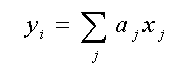
Y = f(X) (1)
is essentially a mapping (Krasnopolsky,
1997) which maps a vector of sensor measurements, X in
Rn, to a vector of
geophysical parameters Y
in Rm. For empirical retrievals, this mapping is constructed
using discrete sets of collocated
vectors X and Y
or matchup data sets {Xp , Yp}.
Single-parameter algorithms
yi = f(X) (2)
may be considered as degenerate mappings
where a vector is mapped onto a scalar (or a vector space onto a line).
This
empirical mapping can be performed using
conventional tools (linear and nonlinear regression) and NNs.
Linear regression is an appropriate tool
for developing many empirical algorithms. It is simple to apply and has
a
well-developed theoretical basis. In the
case of linear regression, a linear model is constructed for transfer function
(TF) f, (2),
(3)This model is linear with respect to both
a
and X , thus it provides a linear approximation of
the TF with respect to X.
The most important limitation of such
a linear approximation is that it works well over a broad range of variability
of the arguments only if the function
which it represents (TF in our case) is linear. If the TF, f,
is nonlinear, linear
regression can only provide a local approximation;
when applied globally, the approximation becomes inaccurate.
Because, TFs are generally nonlinear functions
of their arguments X, linear regression and a nonlinear approximation
with respect to X is often
better suited for modeling TFs. In this case, f can be introduced
as a linear expansion using
a basis of nonlinear functions {jj
}:
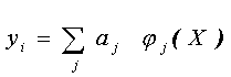 (4)
(4)Finally, nonlinear regression may be applied.
For example, f in (2) can be specified as a complicated nonlinear
function, fNR:
yi = fNR (X, a ) (5)
The expression (4) is nonlinear with respect
to its argument X but linear with respect to the parameters
a.
The nonlinear
regression (5) is nonlinear both with
respect to its argument, X, and with respect to the vector
of regression coefficients, a.
However, in either case, we must specify
in advance a particular type of nonlinear function fNR,
or jj.
Thus, we are
forced to implement a particular type
of nonlinearity a priori. This may not always be possible, because we may
not
know in advance what kind of nonlinear
behavior a particular TF demonstrates, or this nonlinear behavior may be
different in different regions of the
TF's domain. If an inappropriate nonlinear regression function is chosen,
it may
represent a nonlinear TF with less accurcy
than with its linear counterpart.
In the situation described above, where
the TF is nonlinear and the form of nonlinearity is not known, we need
a more
flexible, self-adjusting approach that
can accommodate various types of nonlinear behavior representing a broad
class
of nonlinear mappings. Neural networks
(NNs) are well-suited for a very broad class of nonlinear approximations
and
mappings. Neural networks consist of layers
of uniform processing elements, nodes, units, or neurons. The neurons and
layers are connected according to a specific
architecture or topology. Fig.1 shows a simple architecture which is
sufficient for any continuous nonlinear
mapping, a multilayer perceptron. The number of input neurons, n,
in the input
layer is equal to the dimension of input
vector X. The number of output neurons, m, in the
output layer is equal to the
dimension of the output vector Y.
A multilayer perceptron always has at least one hidden layer with k
neurons.
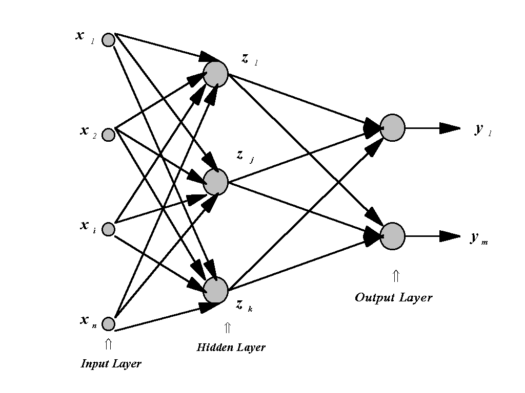
Fig. 1. Multilayer perceptron employing feed forward, fully connected topology.
A typical neuron (processing element) usually
has several inputs (components of vector X), one output,
zj,
and consists
of two parts, a linear part and a nonlinear
part. The linear part forms the inner product of the input vector X
with a weight
vector Wj
(which
is one column of the weight matrix Wji
),
and a bias term, Bj, may also be added. This linear
transformation of the input vector X
feeds into the nonlinear part of the neuron as the argument of an activation
function.
For the activation function, itis sufficient
that it be a Tauber-Wiener (nonpolynomial, continuous, bounded) function
(Chen and Chen, 1995). Here we use a standard
activation function - the hyperbolic tangent. Then, the neuron output,
zj
, can be written as,
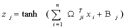
The neuron is a nonlinear element because its output zj is a nonlinear function of its inputs X. Fig. 2 shows a generic neuron.
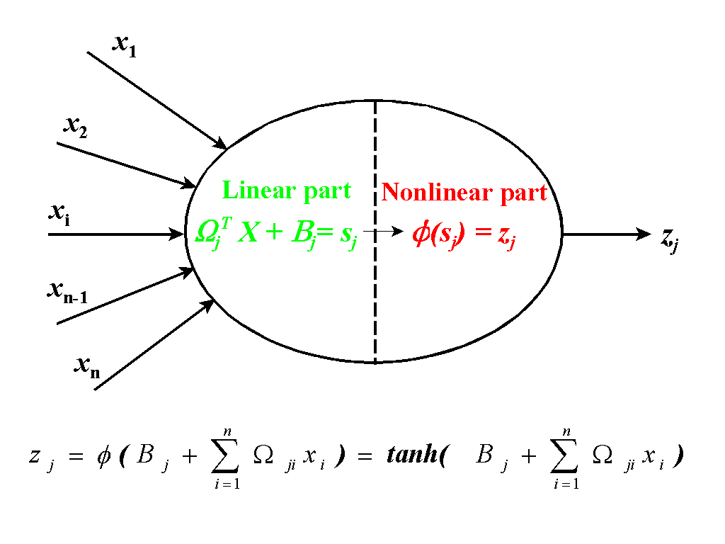
Fig. 2. Generic neuron.
From the discussion above it is clear that
a NN generally performs a nonlinear mapping of an input vector X
in
Rn
(n is the dimension of the input
vector or the number of inputs) onto an output vector Y in
R m (m is the dimension
of the output vector or the number of
outputs). Symbolically, this mapping can be written as,
Y = fNN(X ) (7)
where fNN denotes this neural network mapping (the NN input/output relation).
For the topology shown in Fig. 1 for a
NN with k neurons in one hidden layer, and using (6) for each neuron
in the
hidden and output layers, (7) can be written
explicitly as,
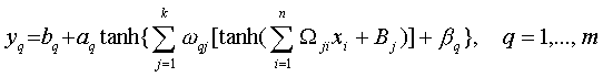 (8)
(8)where the matrix Wji
and
the vector Bj represent weights and biases in the neurons
of the hidden layer; wqj
in Rk×m and
the bqin
Rm represent weights and biases in the neurons of the output
layer; and aq and bq
are scaling parameters. It can
be seen from (8) that any component (yq)
of the NN's output vector Y is a complicated nonlinear function
of all
components of the NN's input vector X.
It has been shown (e.g., Chen and Chen, 1995; Hornik, 1991; Funahashi,
1989;
Gybenko, 1989) that a NN with one hidden
layer (e.g., NN (8)), can approximate any continuous mapping defined on
compact sets in Rn.
Thus, any problem which can be mathematically
reduced to a nonlinear mapping as in (1) or (2) can be solved using
the NN represented by (8). NNs are robust
with respect to random noise and sensitive to systematic, regular signals
(e.g., Kerlirzin and Réfrégier,
1995). NN solutions given by (8) for different problems will differ in
several important
ways. For each particular problem, n
and m are determined by the dimensions of the input and output vectors
X
and Y.
The number of hidden neurons, k,
in each particular case should be determined taking into account the complexity
of the
problem. The more complicated the mapping,
the more hidden neurons that are required. Unfortunately, there is no
universal rule that applies. Usually k
is determined by experience and experiment. In general, if k is
too large, the NN
will reproduce noise as well as the desired
signal. Conversely, if k is too small, the NN is unable to reproduce
the
desired signal accurately. After these
topological parameters are defined, the weights and biases can be found,
using
a procedure called NN training. A number
of methods have been developed for NN training (e.g.,Beale and Jackson,
1990; Chen, 1996). Here we use a simplified
version of the steepest (or gradient) descent method known as the
back-propagation training algorithm. Although
NN training is often time consuming, NN application, after training,
is not. After the training is finished
(it is usually performed only once), each application of the trained NN
is
practically instantaneous and yields an
estimate for (8) with known weights and biases.
Because the dimension of the output vector
Y
may obviously be greater than one, NNs are well suited for modeling
multi-parameter TFs (1). All components
of the output vector Y are produced from the same input vector
X.
They are
related through common hidden neurons;
however, each particular component of the output vector Y
is produced by a separate
output neuron which is unique.
REFERENCES
Beale, R. and T. Jackson,
1990, Neural Computing: An Introduction, Adam Hilger, Bristol, Philadelphia
and New York
Chen, C.H. (Editor
in Chief), 1996, Fuzzy Logic and Neural Network Handbook, McGraw-Hill,
New York
Chen, T., and H. Chen,
1995, "Approximation Capability to Functions of Several Variables, Nonlinear
Functionals and Operators by Radial Basis Function Neural Networks," Neural
Networks, Vol. 6, pp. 904-910,
---,---, "Universal
Approximation to Nonlinear Operators by Neural Networks with Arbitrary
Activation Function and Its Application to Dynamical Systems", Neural
Networks, Vol. 6, pp. 911-917
Funahashi, K., 1989,
"On the Approximate Realization of Continuous Mappings by Neural Networks,"
Neural
Networks, Vol. 2, pp. 183-192
Gybenko, G., 1989,
"Approximation by Superposition of Sigmoidal Functions," in Mathematics
of Control, Signals and Systems, Vol. 2, No. 4, pp. 303-314
Hornik, K., 1991, "Approximation
Capabilities of Multilayer Feedforward Network", Neural Networks,
Vol. 4, pp. 251-257
Kerlirzin, P., P. Réfrégier,
1995, " Theoretical Investigation of the Robustness of Multilayer Perceptrons:
Analysis of the Linear Case and Extension to Nonlinear Networks", IEEE
Transactions on neurl networks, Vol. 6, pp. 560-571
Krasnopolsky, V., 1997,
"Neural Networks for Standard and Variational Satellite Retrievals", Technical
Note, OMB contribution No. 148, NCEP/NOAA