Click here to go to the MMAB home page Global RTOFS Data Analysis with Python

NOTICE: The NOMADS data server address has been changed. The old address
https://nomads.ncep.noaa.gov:9090/
has been changed to
https://nomads.ncep.noaa.gov/
Please update any bookmarks or scripts that use the NOMADS data server.

Home Z-Levels Fronts Sea Ice Metrics WOCE Data Access About

The following example uses Sage Python to extract and visualize the sea surface temperature in the Global RTOFS model using data from the NOMADS data server or a downloaded Global RTOFS NetCDF file.

Prerequisites

The examples make use of the following free software:

1. Python
2. NumPy
3. netcdf4-python: A Python/numpy interface to netCDF
4. Basemap: A module to plot data on map projections with matplotlib

Example: Plot data from the NOMADS Data Server or a NetCDF file

Begin by importing the necessary modules and set up the figure

from mpl_toolkits.basemap import Basemap
import numpy as np
import matplotlib.pyplot as plt
from pylab import *
import netCDF4

plt.figure()

First set up the URL to access the data server. See the Global RTOFS directory on NOMADS for the list of available model run dates.

mydate='20201030';
url='//nomads.ncep.noaa.gov:9090/dods/'+ \
  'rtofs/rtofs_global'+mydate+ \
  '/rtofs_glo_3dz_forecast_daily_temp'

Note that the NOMADS data server interpolates and delivers the data on a regular lat/lon field, not the native model grid. To analyze the model output on the native grid you will have to work from a downloaded NetCDF file (see Example 2), or use a NOPDEF url from the Developmental NOMADS. The latter are experimental links that bypass the grid interpolation step. For example, the NOPDEF URL would be as follows:

mydate='20201030';
url='//nomad1.ncep.noaa.gov:9090/dods/'+ \
  'rtofs_global/rtofs.'+mydate+ \
  '/rtofs_glo_3dz_forecast_daily_temp_nopdef'

It is important to note that if you are using the NOPDEF link, the latitudes and longitudes are returned as arrays, not vectors, and you will be plotting on a tripolar grid, not a regular projection such as Mercator or Lambert Conformal.

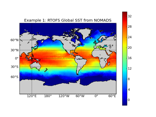
Extract the sea surface temperature field from NOMADS.

file = netCDF4.Dataset(url)
lat  = file.variables['lat'][:]
lon  = file.variables['lon'][:]
data      = file.variables['temperature'][1,1,:,:]
file.close()

Since Python is object oriented, you can explore the contents of the NOMADS data set by examining the file object, such as file.variables.

The indexing into the data set used by netCDF4 is standard python indexing. In this case we want the first forecast step, but note that the first time step in the Global RTOFS OpenDAP link is all NaN values. So we start with the second timestep.

Plot the field using Basemap. Start with setting the map projection using the limits of the lat/lon data itself:

m=Basemap(projection='mill',lat_ts=10, \
  llcrnrlon=lon.min(),urcrnrlon=lon.max(), \
  llcrnrlat=lat.min(),urcrnrlat=lat.max(), \
  resolution='c')

Convert the lat/lon values to x/y projections.

Lon, Lat = meshgrid(lon,lat)
x, y = m(Lon,Lat)

Next, plot the field using the fast pcolormesh routine and set the colormap to jet.

cs = m.pcolormesh(x,y,data,shading='flat', \
  cmap=plt.cm.jet)

Add a coastline and axis values.

m.drawcoastlines()
m.fillcontinents()
m.drawmapboundary()
m.drawparallels(np.arange(-90.,120.,30.), \
  labels=[1,0,0,0])
m.drawmeridians(np.arange(-180.,180.,60.), \
  labels=[0,0,0,1])

Add a colorbar and title, and then show the plot.

colorbar(cs)
plt.title('Example 1: Global RTOFS SST from NOMADS')
plt.show()

You should see this image in your figure window:

---

Example 2: Plot data from an Global RTOFS NetCDF file

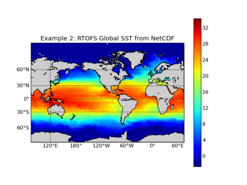
This example requires that you download a NetCDF file from either our NOMADS data server or the Production FTP Server (see our Data Access page for more information. For this exercise, I used the nowcast file for 20111004: rtofs_glo_3dz_n048_daily_3ztio.nc retrieved from NOMADS. This example assumes that the NetCDF file is in the current working directory.

Begin by importing the necessary modules and set up the figure

from mpl_toolkits.basemap import Basemap
import numpy as np
import matplotlib.pyplot as plt
from pylab import *
import netCDF4

plt.figure()

nc='rtofs_glo_3dz_n048_daily_3ztio.nc';

In this example we will extract the surface temperature field from the model. Remember that indexing in Python starts at zero.

file = netCDF4.Dataset(nc)
lat  = file.variables['Latitude'][:]
lon  = file.variables['Longitude'][:]
data = file.variables['temperature'][0,0,:,:]
file.close()

There is a quirk to the global NetCDF files that isn't in the NOMADS data, namely that there are junk values of longitude (lon>500) in the rightmost column of the longitude array (they are ignored by the model itself). So we have to work around them a little with NaN substitution.

lon = np.where(np.greater_equal(lon,500),np.nan,lon)

From this point on the code is almost identical to the previous example. The missing step is that since lat/lon values are arrays in the native grid instead of vectors returned by NOMADS, the meshgrid step is unnecessary.

Plot the field using Basemap. Start with setting the map projection using the limits of the lat/lon data itself (note that we're using the lonmin and lonmax values computed previously):

m=Basemap(projection='mill',lat_ts=10, \
  llcrnrlon=np.nanmin(lon),urcrnrlon=np.nanmax(lon), \
  llcrnrlat=lat.min(),urcrnrlat=lat.max(), \
  resolution='c')

Convert the lat/lon values to x/y projections.

x, y = m(lon,lat)

Next, plot the field using the fast pcolormesh routine and set the colormap to jet.

cs = m.pcolormesh(x,y,data,shading='flat', \
  cmap=plt.cm.jet)

Add a coastline and axis values.

m.drawcoastlines()
m.fillcontinents()
m.drawmapboundary()
m.drawparallels(np.arange(-90.,120.,30.), \
  labels=[1,0,0,0])
m.drawmeridians(np.arange(-180.,180.,60.), \
  labels=[0,0,0,1])

Add a colorbar and title, and then show the plot.

colorbar(cs)
plt.title('Example 2: Global RTOFS SST from NetCDF')
plt.show()

You should see this image in your figure window: