
| Table of Contents |
| STOFS Disclaimer This is an experimental web portal for graphic visualization of the operational and experimental results from the storm surge and tide forecast systems being developed and tested by the National Ocean Service. STOFS model output is NOT total water level guidance. Actual water levels can be significantly higher than forecast due to waves and other components not presently included in STOFS. Please check with your regional National Weather Service forecast office for the official water level forecast. |
||||||||||||||||||||||||||||
| Page
Description: STOFS-3D-Pacific This page provides experimental web dissemination for the output and validation of the 3-D Surge and Tide Operational Forecast System for the Pacific Basin (STOFS-3D-Pacific). The Coastal & Marine Modeling Branch (CMMB) of the Coast Survey Development Laboratory (CSDL) has implemented the new STOFS-3D-Pacific as v3.1. This STOFS-3D-Pacific implementation includes: *3D baroclinic and surface current coverage for the north Pacific basin, from 30 degrees South to the Bering Strait. STOFS-3D-Pacific uses input from the National Water Model and Copernicus’ Global Flood Awareness System (GloFAS) global hydrology to include inland hydrology and extreme precipitation effects on coastal flooding, and also provides surface currents for marine navigation use. The user evaluation and feedback for STOFS-3D-Pacific was officially collected up until January 16 2026, but we will always welcome feedback. The STOFS-3D-Pacific Upgrade Briefing to the NCEP Director occurred on January 22 2026. Operational implementation of STOFS-3D-Pacific v3.1 occurred at the 12 UTC cycle on August 17 2026. Evaluation is always being sought to verify that STOFS-3D-Pacific v3.1 maintains skill in the forecast guidance it provides for your use. Please send your feedback to: Greg Seroka [email] Edward Myers [email] Saeed Moghimi [email] |
||||||||||||||||||||||||||||
| Operational STOFS-3D-Pacific Configuration Model: SCHISM, 3D baroclinic Forcing: GFS and HRRR for surface meteorological forcing (HRRR priority); G-RTOFS as open ocean boundary forcing for subtidal three-dimensional water temperature, salinity, and currents (Copernicus gridded Absolute Dynamic Topography (ADT) satellite altimetry in combination with G-RTOFS for subtidal water level); TPXO9 for tidal forcing; NWM, Copernicus' GloFAS, USGS, and Canadian stream gauge data streamflow Mesh: Pacific Ocean from 30 degrees South to the Bering Strait. Node count: 2,961,412 nodes. Elements count: 5,774,631 (triangular and quadrilateral). Total number of 3-D grid points: 83,839,597. Vertical layers: 34 on average, ranging from 84 near the entrance of Columbia River to just 1 layer in floodplain areas. Resolution: 1.5-2 km near the shoreline, ~300 m for the floodplain, and ~60 m for watershed rivers. Along the U.S. coastline, the land boundary of the domain aligns with the Mean High Water (MHW), except in the Columbia River Estuary and San Francisco Bay, where the land boundary of the domain aligns with the 10-m contour above xGEOID20B, encompassing the coastal transitional zone most vulnerable to coastal and inland flooding. Computation: Computational time step: 90 seconds. In total, STOFS-3D-Pacific currently runs on 3,960 computational cores on Weather and Climate Operational Supercomputing System 2 (WCOSS2). |
||||||||||||||||||||||||||||
| Model
Output Maximal forecasted water level elevation (maxele) on a native netCDF, 6-min forecast water level timeseries at point locations, hourly snapshot fields in GRIB2 format on NDFD subgrids (CONUS West, Alaska, Hawaii, Guam, North Pacific). Digital Output: netCDF and GRIB2 output is available via https://nomads.ncep.noaa.gov/pub/data/nccf/com/stofs/prod/. Graphics Output: this page provides links to reports including map plots of the maximal forecasted water level elevation (maxele), map plots of the maximal forecasted GFS/HRRR winds, timeseries plots of the forecasted combined water levels along with the observed water levels where available, average and individual skill metrics for the point outputs where the observations are available. The reports are generated for operational STOFS-3D-Pacifc. The typical auto-generated model report provides the following information: Name (tag) of the experiment. The tag includes datestamp of the forecast cycle. It is printed on each plot. Please verify that you are looking at the latest cycle by checking the tag. Datestamp when the report was generated (UTC) Date span for the statistical analysis (UTC) Bounding box of the geographical coordinates (East longitudes/North latitudes) The section Maximal Forecasted Water Levels containing the maps of maxele fields for the whole domain and key sub-domains. The section Time-Series Metrics containing the output and the analysis of the water level point output. |
||||||||||||||||||||||||||||
| Skill
Reporting Skill metrics are reported for the time series comparison of the point output against NOAA coastal tide gauges water level observations, where available. The below describes the different metrics. For more details, please see https://github.com/noaa-ocs-modeling/autoval#package-description. Metrics include:
Metrics are computed for each individual point output station. All point output is provided in the Individual Time-Series Statistics sub-section of the report. Below is the example of the time series analysis for a given station, showing the modeled (blue) and observed (green) hydrographs, and the corresponding metrics: 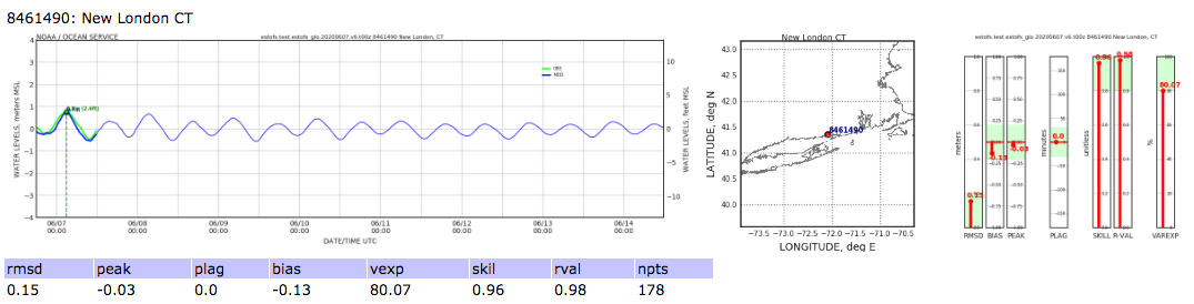 Individual station analysis provides time series skill for the model on the date span where the results overlap the observations. On the example above, the statistics were computed over the 17.8 hours (178 6-minute points where both model and data are valid). Skill metrics is represented as both a text table and a dashboard, with acceptable ranges for each skill shown in green bars. The maps for each skill metrics of all valid individual stations are provided in the experiment report in the Average Time-Series Statistics sub-section of the report. The example below shows the map of RMSE values at each valid station. Values below a 0.2m threshold are plotted as circles. Values above 0.2m are plotted as upward-looking triangles, to help identify areas where the error is larger than a given threshold.  Stations without the observations only report modeled nowcast/forecast time series (blue curve). Average skill metrics for the experiment is shown in the table in the Average Time-Series Statistics sub-section of the report. |
||||||||||||||||||||||||||||
STOFS Pre- and Post-Processing Software The pre- and post-processing software including skill computations has been developed by CSDL, in collaboration with other partners. The codes are written in Python3, and are publicly available from GitHub. The baseline library csdllib. The automated skill analysis application autoval. |
||||||||||||||||||||||||||||
Most Recent Model Output
| ||||||||||||||||||||||||||||