Data Analysis using MATLAB and NCTOOLBOX (Text)

The following examples use MATLAB^® to extract and visualize the sea surface height from RTOFS Atlantic model data from the NOMADS data server and a downloaded GRiB file.

Prerequisites

The examples make use of two free toolboxes,

1. NCTOOLBOX: A MATLAB toolbox for working with common data model datasets
2. M_MAP: A mapping package for MATLAB.

• Example 1: Plot data from the NOMADS Data Server
• Example 2: Plot data from an RTOFS GRiB file

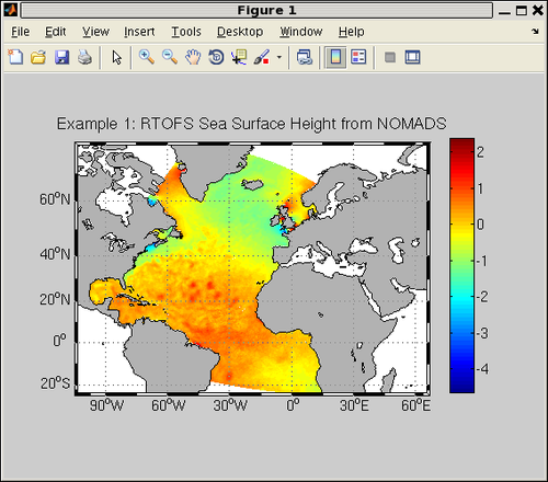
Example 1: Plot data from the NOMADS Data Server

First set up the URL to access the data server. See the RTOFS directory on NOMADS for the list of available model run dates.

mydate='20240427';
url=['http://nomads.ncep.noaa.gov:9090/dods/ofs/ofs',...
   mydate,'/hourly/rtofs_forecast_atl'];

The contents of the OpenDAP dataset can be explored by clicking on the "Info" button in the RTOFS directory for the day or by using this command in MATLAB:

nj_info(url)

Note that the NOMADS data server interpolates and delivers the data on a regular lat/lon field, not the native model grid. To analyze the model output on the native grid you will have to work from a downloaded GRiB file (see Example 2).

Extract the sea surface height field from NOMADS.

nco=ncgeodataset(url);
ssh=nco{'sshgsfc'}(2,1,:,:);
lon=nco{'lon'}(:);
lat=nco{'lat'}(:);

The indexing into the data set is standard MATLAB array indexing. In this case we want the first forecast step, but note that the first time step in the RTOFS OpenDAP link is all NaN values. So we start with the second timestep.

We need to convert the data from single to double precision and remove any singleton dimensions, as the NCTOOLBOX routines return the numbers as they are stored in the netCDF file, in this case single precision.

ssh=double(squeeze(ssh));
lat=double(lat);
lon=double(lon);

Plot the field using M_MAP. Start with setting the map projection using the limits of the lat/lon data itself:

m_proj('miller','lat',[min(lat(:)) max(lat(:))],...
'lon',[min(lon(:)) max(lon(:))])

Next, plot the field using the M_MAP version of pcolor.

m_pcolor(lon,lat,ssh);
shading flat;

Add a coastline and axis values.

m_coast('patch',[.7 .7 .7])
m_grid('box','fancy')

Add a colorbar and title.

colorbar
title('Example 1: RTOFS Sea Surface Height from NOMADS');

You should see this image in your figure window:

---

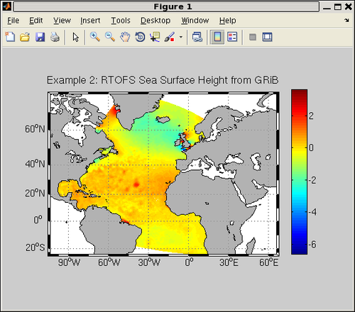
Example 2: Plot data from an RTOFS GRiB file

This example requires that you download a GRiB file from either our NOMADS data server or the Production FTP Server (see our Data Access page for more information. For this exercise, I used the nowcast file for 20111004: ofs_atl.t00z.N000.grb.grib2 retrieved from NOMADS. This example assumes that the GRiB file is in the current working directory.

grib='ofs_atl.t00z.N000.grb.grib2';

Note that the file variables have different names when you access it locally instead of through the OpenDAP interface. Specifically, "sshgsfc" becomes "Sea_Surface_Height_Relative_to_Geoid", "lat" is "Latitude_of_Presure_Point_surface" and "lon" is "Longitude_of_Presure_Point_surface". Once you've defined the ncgeodataset (in this case called nco), you can examine the variable names by printing out the values of nco.variables. Note that since we are working with the model's native grid (Arakawa C-Grid) the lat/lon positions for some values (ssh, temperature, mixed layer depth, others) is different from the lat/lon points for the horizontal velocity components.

nco=ncgeodataset(grib);
nco.variables

And now we extract the SSH field using the parameter names from nj_info:

ssh=nco{'Sea_Surface_Height_Relative_to_Geoid_surface'}(1,1,:,:);
lat=nco{'Latitude_of_Presure_Point_surface'}(:);
lon=nco{'Longitude_of_Presure_Point_surface'}(:);

Note that because each GRiB file has only a single time step I access the first time point, not the second as was the case in Example 1.

From this point on the code is identical to the previous example:

ssh=double(squeeze(ssh));
lat=double(lat);
lon=double(lon);
m_proj('miller','lat',[min(lat(:)) max(lat(:))],...
  'lon',[min(lon(:)) max(lon(:))])
m_pcolor(lon,lat,ssh);
shading flat;
m_coast('patch',[.7 .7 .7]);
m_grid('box','fancy')
colorbar
title('Example 2: RTOFS Sea Surface Height from GRiB');

You should see this image in your figure window:

MATLAB^® is a registered trademark of The Mathworks. Inc.

---

Graphical version of this page

---

Search NWS  

---

About Us
About the MMAB - Mission - Other NCEP Centers - MMAB Personnel - NOAA Locator

Contact Us

USA.gov is the U.S. government's official web portal to all federal, state and local government web resources and services.

---

NOAA/ National Weather Service
National Centers for Environmental Prediction
Environmental Modeling Center
Marine Modeling and Analysis Branch
5200 Auth Road
Camp Springs, Maryland 20746-4304 USA
Comments/Feedback
Disclaimer
Privacy Policy
Page last modified: Tuesday, 28-Jan-2014 17:11:55 UTC