
GOES-8 IMAGERY AS A NEW SOURCE OF DATA TO CONDUCT OCEAN FEATURE TRACKING(1)
Laurence C. Breaker, Vladimir M. Krasnopolsky (General Sciences Corporation/SAIC)
National Centers for Environmental Prediction
and
Eileen M. Maturi
National Environmental Satellite Data and Information Service,
Washington, D.C. 20233-9910
Submitted to Remote Sensing of Environment
April 1999
ABSTRACT
Sequential imagery from the AVHRR has been used to conduct ocean feature
tracking since the early 1980s. One of the primary limitations of AVHRR
data for feature tracking is the lack of temporal continuity, since it
is only possible to obtain coverage from the same satellite once every
12 hours. Thus, for the highly variable flows which are often encountered
in coastal areas, undersampling can be a serious problem. With the availability
of imagery every half hour from the new imager on the GOES-8 and 10 satellites,
the possibility of tracking features on shorter time scales should be considered.
Also, the higher sampling rate of the GOES imager could be particularly
beneficial in obtaining cloud-free coverage of the ocean. However, unlike
the AVHRR which has 1 km resolution, the new imager on GOES has 4 km resolution
in the IR channels. Thus, even for relatively vigorous currents, it will
take at least several hours for a feature to be advected over a distance
of one pixel, and considerably longer to generate displacements which can
be reliably estimated. Also, one of the basic assumptions in conducting
ocean feature tracking has been that it is the sub-mesoscale features that
serve as the primary tracers of the flow. As pixel size increases, the
ability to resolve and track features at these scales clearly comes into
question. Additionally, as with AVHRR imagery, the ability to accurately
navigate successive images is crucial to making reliable estimates of the
feature displacements. These, and other related issues are discussed, and
three examples of feature tracking using imagery from the imager on GOES-8
are presented together with qualitative verifications in each case. Finally,
a new method for rapidly renavigating satellite imagery is presented.
1.0 INTRODUCTION
Although there is a continuing need for real-time information on ocean surface currents in coastal areas, no such information is available to the civilian community on a regular basis for U.S. coastal waters. However, within the oceanographic research community, sequential satellite imagery primarily from the Advanced Very High Resolution Radiometer (AVHRR) and from the Coastal Zone Color Scanner (CZCS) has been used to estimate surface currents in coastal regions. The technique is often referred to as feature tracking since the method depends on tracking the motion of selected features from one image to the next. The same technique has been used by meteorologists since the early 1970s to estimate low-level winds by tracking the motion of selected cloud elements although the time and space scales involved are vastly different. The appeal of ocean feature tracking is that it has the potential of providing synoptic coverage of the surface circulation over relatively large ocean areas on a real-time basis. A detailed discussion of the method for oceanographic applications is presented in Breaker et al. (1994). In the appendix, additional background on feature tracking is included.
One of the primary limitations with AVHRR data for feature tracking is the lack of temporal continuity, since it is only possible to obtain coverage from the same satellite once every 12 hours. Thus for the highly variable flows which are often encountered in coastal areas, undersampling can be a serious problem. The problem is exacerbated in areas where the flow tends to be curvilinear. This occurs because the assumption that must usually be made is that the flow is essentially rectilinear between fixes. As a result, current speeds may be underestimated using this approach. Also, with 12-hour sampling it is not possible to resolve the flow component associated with the semidiurnal tide. With the availability of imagery every half hour from the new imager on the GOES-8 and 10 satellites, the possibility of tracking features on shorter time scales is intriguing. Also, the higher sampling rate on GOES could be particularly beneficial in obtaining coverage of the ocean during brief periods when cloud-free conditions occur.
We proceed to explore the possibility of using imagery from the GOES
imager to conduct ocean feature tracking. As part of this activity, we
present several examples of feature tracking which are preliminary in nature
using this new source of information. We also introduce some of the issues
and problems related to feature tracking with this new source of data.
Finally, a method for quickly and efficiently renavigating satellite imagery
is presented.
2.0 SENSOR CHARACTERISTICS
The characteristics of the new GOES imager which are relevant to feature
tracking include the wavelength regions which can be exploited, the number
of digitization levels, the spatial resolution of the instrument, the accuracy
to which the imagery can be navigated, and the repeat cycle to obtain coverage
over the same area. The imager has five spectral bands, three of which
are expected to be useful for ocean feature tracking, the visual band (0.52
to 0.72 microns), and the two far IR bands, (10.2 to 11.2 microns and 11.5
to 12.5 microns; the spectral bands for the GOES imager are similar to
those employed by the AVHRR). The new imager also has 10-bit digitization
in both the IR and visible bands. The spatial resolution of the instrument
for the visual channel is ~1 km based on the instantaneous geometric field
of view (IGFOV) (Menzel and Purdom, 1994). For the IR channels, the IGFOV
is ~4 km at nadir. Earth location accuracy is nominally in the range of
2-4 km, but degrades slightly between noon (~4 km) and midnight (~6 km).
In any case, successive images will have to be renavigated using known
landmarks in order to achieve the accuracy required for feature tracking
(i.e., < 4 km). Although imagery from the GOES imager can be obtained
as frequently as once per every half hour, it is doubtful that it can be
used more frequently than every 4-6 hours, based on the expected scales
of motion. Overall, the improvements and upgrades which have been added
to the new imager on GOES-8 create sharper and cleaner images which make
it easier to detect both meteorological and oceanographic features in comparison
to the imagery obtained from the previous GOES satellites, according to
Ellrod et al.(1998). These results clearly have a positive impact on the
feature tracking problem.
3.0 FEATURE TRACKING: EXAMPLES AND ISSUES
3.1 Examples
Software, originally developed to conduct feature tracking employing AVHRR imagery, was modified to ingest and display imagery from the GOES imager. This modified software was implemented on an HP 7000 workstation and three examples of feature tracking have been prepared using selected image pairs from the GOES-8 satellite. In each case, the spectral band from 10.2 to 11.2 microns was used. The feature tracking has been performed interactively by manually selecting suitable features whose identity could be clearly established in both images for each pair. Because this was the first time, to our knowledge, that imagery from the GOES-8 (or GOES-10) geostationary satellite has been used to conduct ocean feature tracking, we felt that manual supervision was essential. Also, the analyst who conducted the feature tracking, although familiar with image analysis techniques, was not a trained oceanographer and so had no preconceived notions as to what the flow fields should look like. Finally, no renavigation of the images has been performed; however, only images with coregistration errors of one pixel or less were used in this feature tracking exercise.
Fig. 1 Fig. 2
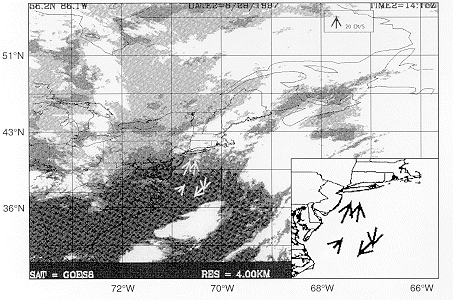
Fig. 3
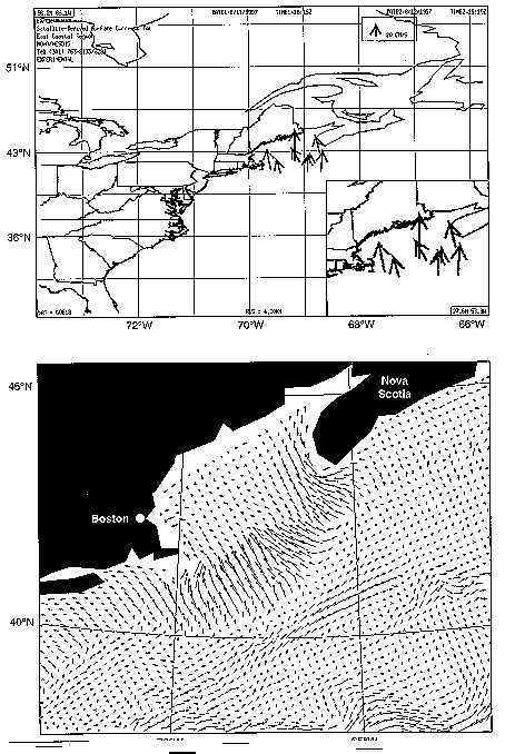
Figure 1. The top panel (a) depicts a cyclonic pattern of flow in the Gulf of Maine in a satellite image acquired from GOES-8 on August 25 and 26, 1997, which is generally consistent with the expected seasonal circulation in this region. The middle panel (b) shows a feature tracking analysis with similar results obtained using AVHRR imagery from August 22 and 23, 1993. The bottom panel (c) shows the expected surface circulation in the Gulf of Maine for late summer taken from the climatology of Bumpus and Lauzier (1965).
Figure 2. The top panel includes eight surface velocity vectors which indicate surface flow into the Gulf of Maine most likely reflecting the influence of the incoming, i.e., flood, tide. A blowup of the area is shown in the lower right-hand corner. A velocity scale is included in the upper right-hand corner. The images from GOES-8 were acquired on August 11 and 12, 1997. The lower panel displays surface flow vectors from a coastal circulation model that includes tidal forcing for March 1, 1995 at 2100 UTC. Again, inflow into the Gulf of Maine is depicted, similar to the pattern produced from the GOES-8 imagery. For further details concerning this comparison, see the text.
Figure 3. Five surface flow vectors are shown which were derived from
GOES-8 imagery acquired on August 28 and 29, 1997. A
blowup of the area is shown in the lower right-hand corner. The
three surface flow vectors on the continental shelf which are closest to
the coast indicate flow to the NE, consistent with climatological wind
forcing in the region. The two surface flow vectors further offshore appear
to be located in the Slope Water region between the shelf and the Gulf
Stream. The prevailing flow in this area is consistently to the SW and
so the satellite-derived flows are generally consistent with the expected
flow in this area.
The first example applies to the Gulf of Maine (Fig. 1a), where images were acquired on August 25 and 26, 1997 at 1315 UTC. The origins of the vectors are plotted at the mid-points between the estimated positions of the features which were used to track the motion. Here, a cyclonic pattern of surface flow can be inferred, which is consistent with the expected cyclonic circulation that occurs in this region and is particularly well-developed during the summer months (e.g., Bigelow, 1927). Fig.1c, taken from the atlas of Bumpus and Lauzier (1965), shows the cyclonic pattern of flow for the Gulf of Maine (summer/autumn) which can also be seen in the flow vectors obtained from the GOES-8 imagery. Similar results were obtained by Breaker et al. (1994; Fig. 1b), who compared flow fields obtained using AVHRR imagery with the same climatology. Surface currents in the Gulf of Maine are generally weak, on the order of 15 cm/sec or less (Bumpus,1973). Due to the lack of resolution it is difficult to estimate flow speeds reliably from our results but generally they appear to be of the same order(2). Because the images were 24 hours apart it is not possible to distinguish the effects of the semidiurnal tide which predominates in this region (Redfield,1958).
The second example, again taken from the Gulf of Maine, is based on images acquired at 1615 UTC on August 11, 1997, and at 1915 UTC on August 12, 1997. The resulting eight surface flow vectors are shown in Fig. 2 (top panel). A blowup of the area is shown in the lower right-hand corner. These flow vectors are generally located near the entrance of the Gulf of Maine in the vicinity of Georges Bank. They indicate flows of ~20 - 40 cm/sec into the Gulf and are most likely due to the incoming tide. Amplification of the currents, in particular, is expected as the incoming tide propagates from the deeper waters offshore to the relatively shallow waters over Georges Bank. In the lower panel of Fig. 2, we have included surface currents from an experimental coastal ocean circulation model which includes forcing from the diurnal and semidiurnal tides (Kelley et al., 1997). Clearly, the speeds are much higher over Georges Bank and the directions are generally similar to those obtained from the GOES-8 imagery. According to tide tables for the Atlantic coast (U.S. Department of Commerce, 1999), maximum tidal currents over Georges Bank range from about 50 to over 100 cm/sec at flood. We note that the speeds obtained from the satellite imagery in this case reflect the net displacements of thermal features which have been tracked over a period of 27 hours and so should not be compared directly with instantaneous values obtained from other sources.
The third example covers a portion of the mid-Atlantic Bight between
Cape Hatteras and Long Island (Fig. 3). These images were acquired on August
28 and 29, 1997 at 1415 UTC. The three surface flow vectors closest to
the coast are located on the continental shelf approximately midway between
the coast and the continental margin. They most likely reflect the response
to wind forcing which is consistently from the southwest during summer
(e.g., Thompson and Hazen, 1983). The surface circulation along the shelf
in the mid-Atlantic Bight is responsive to surface wind forcing on synoptic
time scales, an observation which has been confirmed repeatedly (e.g.,
Beardsley and Boicourt, 1981). Speeds in this case are in the range of
10-25 cm/sec. The two flow vectors further offshore are apparently located
in the Slope Water region which lies between the continental shelf and
the Gulf Stream. Flow in the Slope Water region west of ~65W is essentially
cyclonic with waters closer to the shelf margin flowing consistently to
the southwest at speeds of ~15 cm/sec (Csanady and Hamilton, 1988). Numerous
drifter studies associated with the 106-Mile Deepwater Municipal Dump Site
located southeast of New York harbor have confirmed the net southwesterly
flow in this region (e.g., Aikman and Wei, 1995). Thus, both the speeds
and directions of these image-derived flow vectors from GOES-8 are generally
consistent with the expected circulation in this area.
3.2 Issues
There are a number of issues that should be considered in using imagery from the GOES-8 and 10 satellites to conduct satellite feature tracking. Because imagery can be obtained as often as once every half hour from the GOES imager, the possibility of exploiting transient gaps in cloud cover to obtain clear views of the ocean surface is potentially important. However, the spatial resolution of the imager in the IR channels is approximately 4 km, significantly lower than the 1 km resolution for the IR channels on the AVHRR. As a result, for a given velocity it will take much longer to advect a water parcel over the distance of one pixel. Based on our experience in using AVHHR imagery to conduct feature tracking, feature motions of at least several pixels are required in order to estimate displacements reliably. Errors in earth location are particularly troublesome in this regard, and often dictate how small an interval between images can be tolerated. If we take the published figure of 4 km for the error amplitude in earth location accuracy for the imager (see previous section), then to obtain a signal-to-noise ratio of 3, a feature displacement of at least 12 km would be required. For a current speed of 15 cm/sec, this in turn would require a time separation between images of more than 20 hours to obtain a displacement large enough to be reliably estimated. It is important to realize that longer separation times may be required between images from GOES due to the increase in pixel size and/or lower current speeds. However, the potential of half hourly sampling should still be advantageous in obtaining cloud-free coverage, since two images, 20 hours apart, could potentially be acquired every half hour. On the negative side, if the sampling intervals become too long, the differences between curvilinear motion, which may actually occur, and rectilinear motion, which must be assumed, can result in significant underestimates of the true current speed. Finally, with respect to pixel size, one of the basic assumptions in conducting ocean feature tracking is that it is the sub-mesoscale features that serve as the primary tracers of the flow (Njoku et al., 1985). As pixel size increases, the ability to resolve and track features at these scales comes into question. Clearly where the flow is coherent over distances which are large compared to the pixel size, the lower spatial resolution will present less of a problem.
As indicated in section 2, navigation accuracy for the GOES imager decreases slightly between noon and midnight. This degradation in navigation accuracy could be important for the bands which are used to conduct feature tracking. Navigation statistics for the GOES imagers are produced routinely by the NESDIS Office of Satellite Operations. These statistics indicate the percent of time that imager products remain within specified limits for navigation accuracy (accuracy specifications for the IR bands is ± 6 km, and for the visual band it is ± 4 km). These statistics show that navigation accuracy for the imager are acceptable 98% of the time for visible imagery, and 93% of the time for IR imagery (Pinkine, personal communication). As a result, the imagery, at least in some cases, will have to be renavigated in order to conduct feature tracking. As with AVHRR imagery in the past, this renavigation can be accomplished using landmarks as anchor points to best fit the images to these known locations using the method of least squares (e.g.,Krasnopolsky and Breaker,1994). Image renavigation is usually a time-consuming task since the computation requires that the locations of all pixels in each image be adjusted. To reduce the time required to renavigate the GOES imagery, a new method for navigating satellite data is presented in the appendix. The velocity vectors themselves are corrected for navigational errors in this approach. The application of this method results in a major reduction in computing time which is directly proportional to the size of the images involved. The method is general and so is clearly applicable to other sources of satellite data as well.
Although the GOES imager has 5 spectral bands, only the two IR bands
between 10.2 and 12.5 microns, and the visual band between 0.52 to 0.72
microns will most likely be useful for feature tracking. The primary concern
is to obtain imagery which detects the features with sufficient signal-to-noise
ratio, and delineates them with the greatest clarity. Any process that
reduces the clarity of the features such as remapping, interpolation to
another grid, or combining bands will degrade our ability to conduct feature
tracking. In the examples presented here, the IR band between 10.2 and
11.2 microns was used. Although we have not, as yet, made any detailed
comparisons, it is our expectation that there will be no significant difference
between this band and the adjacent IR band (i.e., 11.5 to 12.5 microns)
as far as our ability to conduct feature tracking is concerned. Of particular
interest is the possibility of exploiting the visual band for feature tracking
because of its higher spatial resolution (1 km). Past experience with visual
imagery from the AVHRR indicates that in certain coastal regions it should
be possible to detect and track features associated with freshwater outflows
from various rivers and coastal embayments. Although the spectral resolution
of the visual band on the GOES imager is relatively low (compared to the
widths of the spectral bands for the CZCS or the ocean color sensor on
SeaWiFs), its higher spatial resolution means that the time separation
between images can be reduced which will almost certainly provide better
estimates of the current speeds. Areas such as the mouths of the Cheaspeake
and Delaware Bays, and the New York Bight are regions which are likely
candidates for feature tracking using visual imagery from GOES-8.
4.0 CONCLUDING COMMENTS
The results presented here are preliminary in nature. We believe that
they are unique in the sense that such measurements have either not been
made, or at least not reported, before. In the three cases considered,
the flow speeds and flow directions are generally consistent with what
is known about the circulation in each of the areas where estimates of
surface motion were obtained. However,
it is imperative that measurements of surface flow made using imagery from
the GOES imager be validated through side-by-side comparisons with in situ
measurements of surface motion using devices such as drifting buoys, drogues,
etc. Although it is difficult to make such comparisons it is the only way
to establish the credibility of this technique together with the data it
employs. As mentioned in the introduction, the temporal sampling capability
of the new GOES imager is probably sufficient to meet the needs of the
oceanographic community. However, unlike the AVHRR which has 1 km spatial
resolution in the IR bands, the imager has 4 km resolution, a potential
limitation for oceanographic applications such as feature tracking. At
the present time there is no single satellite instrument that is ideally-suited
to conduct ocean feature tacking: either the temporal sampling is not sufficient
or the spatial resolution is too low. On the horizon is a new instrument
called the Special Events Imager (SEI) which will be flown aboard future
GOES satellites starting with GOES-N or -O (ca. 2002). According to Brown
and Esaias (1999), the SEI will acquire multispectral observations of high
spatial, radiometric, and spectral resolution. It will be able to acquire
imagery every 10 minutes with a spatial resolution of 300 meters. This
instrument will be particularly well-suited to conduct ocean feature tracking
because of it's spatiotemporal sampling capabilities. Finally, we
believe that the results presented here (1) are encouraging and demonstrate
the possibility of using imagery from the new imager on GOES-8 (and 10)
for conducting ocean feature tracking, and (2), may provide further guidance
in developing a fully adequate methodology to conduct ocean feature tracking
in
the future as new instruments such as the SEI are developed .
5.0 ACKNOWLEDGMENTS
The authors would like to thank Jamie Hawkins and Kent Hughes of the
National Environmental Satellite and Data Information Service (NESDIS)
for supporting this work in the past. Nick Pinkine, of NESDIS, is also
thanked for providing helpful information on navigation statistics for
the GOES-8 satellite. We would also like to acknowledge the helpful comments
which were provided to us by the reviewers who were anonymous.
APPENDIX
A TECHNIQUE FOR RAPIDLY CORRECTING EARTH LOCATION ERRORS WITH APPLICATION TO SATELLITE FEATURE TRACKING
a. Feature tracking background
Satellite feature tracking is usually accomplished by measuring the displacement of selected ocean thermal or visible features (or patterns) between successive satellite images which have been spatially aligned or coregistered. In feature tracking, if a unique feature can be identified in two successive satellite images and its coordinates determined, then the displacement and the velocity vectors of the feature can be expressed approximately as
D = (Du , Dv) = Du i
+ Dv j
(1)
V = D / Dt
(2)
D = R2 - R1 and Dt = t2 - t1 (3)
where i and j are unit vectors, and
R1 = (u1,v1) and R2
= (u2,v2) are the coordinates of the feature
at times t1 and t2. More precisely,
D
should be calculated as the great circle distance over the surface of the
earth. However, for the small displacements that are usually encountered
in practice (< 100 km), the curvature of the Earth can be neglected,
and (1) - (3) give a displacement error of less than 0.002% (2 meters).
This error is negligible compared to the other sources of error which arise
in estimating the velocity vectors.
b. Errors in feature tracking
Many sources of error contribute to the errors in estimating the displacement
D
(1) and velocity V (2) (Krasnopolsky and Breaker, 1994).
We can express D as
D = d + q (4)
q = q0 + qn + qph
(5)
where d is an exact displacement and q is an error in the displacement which has at least three components. An uncorrectable error q0, equal to the resolution of the image, |q0| = R0, is introduced in the displacement because of the finite resolution of the imagery. The third term in (5), qph, is a contribution due to the physical processes which affect the observed changes (changes in shape and size of the tracked feature during the time interval between successive images due to local thermodynamical effects) in displacement but have not been taken into account. These changes do not represent true surface motion, but do introduce an error, qph, in the measured displacement. To estimate this term requires the application of a physical model which takes into account the physical processes involved (e.g., Wahl and Simpson, 1990).
The second and probably most important contribution to (5), qn, is due to the error in earth location. The measured coordinates of the feature are degraded by navigational errors which can be written as (Krasnopolsky and Breaker, 1994)
Ri = ri + ei, (6)
where the vectors ri = (xi,yi), ei = (exi,eyi), i = 1,2, are the exact coordinates and earth location errors of the feature in the first and second images, respectively. From (3), (4) and (6), we can obtain an expression for the measured displacement D = d + q where the vectors d and qare
d = r2 - r1 = (x2
- x1 , y2 - y1); q
= e2 - e1=
(ex2 - ex1
,e y2 -ey1)
(7)
d is an exact displacement and q is the
displacement error due to earth location
errors contained in (6). The error in the displacement, q,
can, in turn, be estimated as
||e1| - |e2||
< |q| < |e1|
+ |e2|
(8)
Earth location errors, e1,2,
in AVHRR imagery may reach magnitudes as high as 15 km (Krasnopolsky and
Breaker, 1994) with the errors in the derived velocity (t
= q / Dt) approaching 35 cm/sec when
the images are 24 hours apart. Therefore, in coastal areas when the surface
flows are sufficiently weak ( < 25 cm/sec), the errors in the derived
velocities caused by errors in earth location may reach 100% or more.
c. Correcting earth location errors.
The standard method of correcting earth location errors, based on adjusting the locations of all pixels in both images is time consuming because it first involves registration of the images to a map base followed by shifting all image pixels to their correct positions and eliminating any distortions caused by the shifting. This procedure must be done twice (once for each image) in order to complete the task.
Here we introduce an alternative method for correcting earth location errors, based on relative navigation or coregistration of the two images, a procedure which is well-suited for feature tracking, and permits us immediately to correct the derived field (displacement or velocity ) without the need to renavigate both images. This procedure allows us to reduce, by up to a factor of 10, the time required to correct the errors in earth location.
The standard way to correct earth location errors is to correct both
images for earth location before feature tracking is performed. The correction
function F(R) = (F(u,v), G(u,v)) is introduced for
each of the images, which transforms the uncorrected coordinates to their
correct values (Krasnopolsky and Breaker, 1994)
ri = Ri + F(Ri),
i
=
1,2
(9)
The first step is to register the images to a map base and to estimate
the navigation errors. Several (usually > 6) landmarks or Ground Control
Points (GCPs) are used for this purpose. Coordinates of these GCPs are
determined from the image and from a high resolution map or database and
are used to estimate the errors and calculate the correction functions
F
(Krasnopolsky and Breaker, 1994). Next, the corrections
F
are applied (9) N × M times for each image (N and M
are
the image dimensions) to shift each pixel to the correct position. The
time needed to renavigate two images can be estimated as
T = 2 ( t1 + t2); t1 = tc k; t2 = tsh N M (10)
where tc is the time required for processing one GCP and tsh is time required to shift one pixel of the image to its correct position. This procedure is clearly time consuming. For example, using a DEC workstation (VAXstation 4000), t1 3 - 5 min (to process 10 - 15 GCPs) and t2 20 min (for N = M = 512). Therefore, it takes about one hour to correct both images for navigational errors, using this approach.
Here, an alternative approach is introduced which is much less time
consuming. To begin, substitute (9) in (7) to obtain the exact displacement
d:
d = R2 - R1 + (F(R2)
- F(R1)) = D + (F(R2)
- F(R1)) (11)
If we consider navigational errors with low spatial and/or temporal
frequencies (see Krasnopolsky and Breaker, 1994), (11) can be written as
d = D + G(R)
(12)
where d is the exact displacement, D is
the displacement degraded by navigational errors, and
G(R)
= (f(u,v), g(u,v)) is a correction function, which corrects the navigational
errors in displacement and where R
(R1 , R2). Without loss of generality,
we can assume that R = (R1 +
R2)/2.
A simple condition can be applied to determine this correction function,
namely that the displacements for the GCPs must be equal to zero, or
DGCP + G(R) = 0 , or G(R)
= - DGCP
(13)
The technique described in Krasnopolsky and Breaker (1994) can be applied directly to obtain the solution of (13); the correction function can be approximated by polynomials and the coefficients of the polynomials can be found using the method of least squares.
To better understand the difference between the standard approach and
the new approach, and to estimate the time needed to correct the navigation
in the second case, let us formulate this algorithm which has just been
described (eqs. 12-13) step by step: (1) select several GCPs which are
clearly visible in both images, (2) determine the observed displacements
of the GCPs, DGCP, (3) solve (14) to determine
the correction function G(R), (4) determine the observed
displacements of a selected feature, D, (5) determine the
exact displacement d, by applying (12). The time needed to
renavigate n features can now be estimated as
Tnew = t1 + t3 ; t1
=
tc k;
t3
= tcf n
(14)
where tc is the time required for processing one GCP (the same as in (10)) and tcf is the time required to apply the correction function,
tcf = tsh/
2
(15)
This approach does not shift the pixels of the images involved and does
not require time to correct for any distortions introduced by such shifts.
As mentioned above, for a DEC workstation (VAXstation 4000), t1
3 - 5 min and t2 20 min for an image with 512 by 512
pixels (N = M = 512 in eq.(10)). The ratio t3/t2
can
be estimated from (10), (14) and (15):
t3 / t2 = n / (2 N
M)
(16)
The number of features processed in a given feature tracking exercise
can reach n = 100. Therefore, in this case, t3 / t2
0.0002 and t3 0.3 sec. Thus, t3 can
be neglected in comparison to t1, and so for Tnew,
we obtain
Tnew t1 5 min
Thus, the new approach allows us to reduce the most time consuming part
of the renavigation process significantly,
i.e., reducing the time required to correct earth location errors by up
to a factor of 10.
6.0 REFERENCES
Aikman,F. and E.J. Wei, "A comparison of model-simulated trajectories
and observed drifters in the mid-Atlantic Bight", J. Marine Env. Engg.,Vol.
2, pp.123 - 139, 1996.
Beardsley,R.C. and W.C. Boicourt, "On estuarine and coastal shelf circulation
in the mid-Atlantic Bight", In Evolution of Physical Oceanography, ed.
B.A. Warren and C. Wunsch, pp.198-233. MIT Press, Cambridge, MA, 1981.
Bigelow, H.B., Physical oceanography of the Gulf of Maine, Bulletin
of the U.S. Bureau of Fisheries 40, pp.511- 1027, 1927.
Breaker, L.C., V.M. Krasnopolsky, D.B. Rao and X.H. Yan. "The feasibility
of estimating ocean surface currents on an operational basis using satellite
feature tracking methods", Bull. Amer. Meteor. Soc., Vol. 75, pp.
2085 - 2095, 1994
Brown,C.W. and W.E. Esaias,"NOAA & NASA propose new mission", backscatter,
Vol. 10, p.25, 1999.
Bumpus,D.F., "A description of the circulation on the continental shelf
of the east coast of the United States", Progress
in Oceanography, Vol. 6, Pergamon Press, pp.111 - 157,1973.
Bumpus,D.F. and L.M.Lauzier, "Surface circulation on the continental
shelf off eastern North America between Newfoundland and Florida", Serial
Atlas of the Marine Environment, American Geographical Society, Folio 7,
Plate 8, 4 pp.,1965.
Csanady, G.T. and P. Hamilton, "Circulation of slopewater", Continental
Shelf Research, Vol. 8, pp. 565-624, 1988.
Ellrod,G.P., R.V.Achutuni, J.M.Daniels, E.M.Prins and J.P.Nelson, "An
assessment of GOES-8 imager data quality", Bull. Amer. Meteor. Soc.,
Vol. 79, 2509 - 2526, 1998.
Kelley, J.G.W., F. Aikman, L.C. Breaker and G.L. Mellor, "Coastal Ocean
Forecasts, Real-time Forecasts of Physical State of Water Level, 3-D Currents,
Temperature, Salinity for U.S. East Coast". Sea Technology, Vol.
38, pp. 10-17, 1997.
Krasnopolsky, V.M. and L.C. Breaker. "The Problem of AVHRR Image Navigation
Revisited,"
Int. J. Remote Sensing, Vol. 15, pp. 979 - 1008, 1994
Menzel, W.P and J.F.W. Purdom. "Introducing GOES-I: the first of a new
generation of geostationary operational environmental satellites", Bull.
Amer. Meteor. Soc., Vol. 75, pp. 757 - 781, 1994.
Njoku,E.G., T.P.Barnett, R.M.Laurs and A.C.Vastano, "Advances in satellite
sea surface temperature measurements and oceanographic applications", J.
Geophys .Res., Vol. 90, pp.11573 - 11586, 1985.
Pinkine, N. "GOES image navigation and registration statistics", Facsimilemessage,
NOAA, National Environmental Satellite, Data, and Information Service,
16 pp., 1997
Redfield,A.C., "Influence of the continental shelf on tides of the Atlantic
coast of the United states", J. Mar. Res., Vol. 17, 432-448, 1958.
Thompson, K.R. and M.G. Hazen,"Interseasonal changes of wind stress
and Ekman upwelling: North Atlantic, 1950-1980", Can. Tech. Rep. Fish.
Aquat. Sci. 1214, 175 pp., 1983.
U.S.Department of Commerce, "Current Tables Atlantic Coast North America",
U.S. Department of Commerce, NOAA, pp. 179, 1999.
Wahl ,D.D. and J.J.Simpson. "Physical processes affecting the objective
determination of near-surface velocity from satellite data", J. Geophs.
Res., Vol. 95, pp. 13511 - 13528, 1990
2. - Although not shown in Figure 1a, a velocity scale, included in the original figure from which the blow-up in Fig. 1a was taken, was used to estimate these flow speeds.